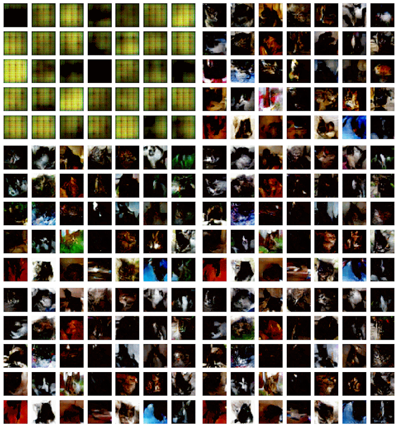
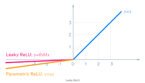
Source From Here
Introduction
Generative Adversarial Networks, or GANs for short, are some of the most potent tools a machine learning practitioner can use. GANs are capable of doing everything from super-resolution in images, to image translation, to facial manipulation, to medicine creation, to much, much more.

In this article, we will cover both the intuition behind how GANs work, and how we can implement them in Keras. Specifically, we will be first implementing a fully-connected GAN (FCGAN) for MNIST, then later improving that into a deep convolutional GAN (DCGAN) for a class of CIFAR-10.
The completed code we will be creating in this tutorial is available on my GitHub, here.
How GANs Work
A GAN works by battling two neural networks, a generator and a discriminator, against each other in an attempt to learn the probability distribution of a dataset. The generator, often written as G, attempts to create realistic-looking images. It does this by taking some noise vector, z, and applying a series of calculations on it; these calculations usually take the form of a neural network. The result is G(z), an image that is the generator’s attempt to fool the discriminator; On the other hand, the discriminator, D, attempts to classify real and fake images. Images are considered “fake” if the generator creates them, and “real” if they were selected from the dataset. x represents the input image, and D(x) represents the probability that the discriminator believes x is real.

Adapted from source
As the discriminator improves at classifying real vs. fake images, it forces the generator to improve at creating images. The goal is for the generator to become so adept at creating images that the generated images are indistinguishable from reality, meaning even a perfect discriminator would never be sure about the validity of the images, i.e. D(x)=0.5.
If you would like a much more detailed explanation of the math behind GANs, I would recommend reading the original paper by Goodfellow et al.
Putting it into Practice
Training a GAN is a lot harder than understanding how it works. While I will walk through the Keras code to create a simple GAN, I recommend following roughly what I do instead of copying it verbatim. Finding the correct architecture for GANs is a challenging task, and the best way to gain intuition about building models is through trial and error. (original notebook)
Setting Everything Up
Let’s start by defining a few hyperparameters:
- from keras.optimizers import Adam
- from keras.models import load_model
- import numpy as np
- import os
- np.random.seed(10)
- noise_dim = 100
- batch_size = 16
- steps_per_epoch = 3750
- epochs = 10
- save_path = 'fcgan-images'
- img_rows, img_cols, channels = 28, 28, 1
- optimizer = Adam(0.002, 0.5)
- gan_model_serialized_path = "mnist_gan_model.h5"
- gan_gen_model_serialized_path = "mnist_gan_model_gen.h5"
- gan_dsm_model_serialized_path = "mnist_gan_model_dsm.h5"
After setting the hyperparameters, we can load the dataset of our choice:
- from keras.datasets import mnist
- import os
- (x_train, y_train), (x_test, y_test) = mnist.load_data()
- x_train = (x_train.astype(np.float32) - 127.5) / 127.5
- x_train = x_train.reshape(-1, img_rows*img_cols*channels)
- if not os.path.isdir(save_path):
- os.mkdir(save_path)
As we implement an FCGAN, we will be loading mnist into a flat shape; however, we will replace this when we implement a DCGAN. If we were to generate, let’s say faces, we would replace this section with the code to load those faces into the same format.
Creating the Generator
Now it’s time to define a function to create the generator. This is the part of the model that is most creative, and I highly encourage you to invent your own architectures:
- from keras.models import Sequential
- from keras.layers import Dense
- from keras.layers.advanced_activations import LeakyReLU
- def create_generator(noise_dim=noise_dim, optimizer=optimizer):
- if os.path.isfile(gan_gen_model_serialized_path):
- return load_model(gan_gen_model_serialized_path)
- generator = Sequential()
- generator.add(Dense(256, input_dim=noise_dim))
- generator.add(LeakyReLU(0.2))
- generator.add(Dense(512))
- generator.add(LeakyReLU(0.2))
- generator.add(Dense(1024))
- generator.add(LeakyReLU(0.2))
- generator.add(Dense(img_rows*img_cols*channels, activation='tanh'))
- generator.compile(loss='binary_crossentropy', optimizer=optimizer)
- return generator

We must use the tanh activation for the final layer to stay consistent with our normalization of the images earlier, and for better results.

The optimizer we use is also very important. If we had a learning rate of just a bit too high, the model would enter mode collapse, where it would no longer be able to improve, and would produce garbage images.
Creating the Discriminator
Next up, the discriminator. Again, I recommend playing around with the architecture and seeing what results you get:
- def create_discriminator(optimizer=optimizer):
- if os.path.isfile(gan_dsm_model_serialized_path):
- return load_model(gan_dsm_model_serialized_path)
- discriminator = Sequential()
- discriminator.add(Dense(1024, input_dim=img_rows*img_cols*channels))
- discriminator.add(LeakyReLU(0.2))
- discriminator.add(Dense(512))
- discriminator.add(LeakyReLU(0.2))
- discriminator.add(Dense(256))
- discriminator.add(LeakyReLU(0.2))
- discriminator.add(Dense(1, activation='sigmoid'))
- discriminator.compile(loss='binary_crossentropy', optimizer=optimizer)
- discriminator.trainable = False
- return discriminator
Building the GAN
With the discriminator and generator in place, we can create the combined GAN model. First, we can initialize the discriminator and generator with:
- discriminator = create_discriminator()
- discriminator.summary()
Then is for generator:
- generator = create_generator()
- generator.summary()
Then, we can use a little trick; we can set discriminator.trainable to False. Why would we want to do this?
Well, we aren’t going to be training the generator model directly — we are going to be combining the generator and discriminator into a single model, then training that. This allows the generator to understand the discriminator so it can update itself more effectively.
Setting discriminator.trainable to False will only affect the copy of the discriminator in the combined model. This is good! If the copy of the discriminator in the combined model were trainable, it would update itself to be worse at classifying images. We’ll look more into this when we train the model.
To combine the generator and discriminator, we will be calling the discriminator on the output of the generator.
- from keras.layers import Input
- from keras.models import Model
- gan_input = Input(shape=(noise_dim,))
- fake_image = generator(gan_input)
- gan_output = discriminator(fake_image)
- gan = Model(gan_input, gan_output)
- gan.compile(loss='binary_crossentropy', optimizer=optimizer)
- gan.summary()
This gives us a model that takes some random noise, z, as input, and returns how convinced the discriminator is that the generator’s images are real, D(G(z)) . Specifically, it has an input shape of (None, 100) and an output shape of (None, 1). The 100 in the input shape comes from noise_dim.
Training the GAN
Now comes the time to put the GAN training into action. Since we are training two models at once, the discriminator and the generator, we can’t rely on Keras’ .fit function. Instead, we have to manually loop through each epoch and fit the models on batches:
- for epoch in range(epochs):
- for batch in range(steps_per_epoch):
- ...
- noise = np.random.normal(0, 1, size=(batch_size, noise_dim))
- fake_x = generator.predict(noise)
We can create our real_x data by sampling random elements from our x_train that we loaded earlier:
- real_x = x_train[np.random.randint(0, x_train.shape[0], size=batch_size)]
- x = np.concatenate((real_x, fake_x))
- disc_y = np.zeros(2*batch_size)
- disc_y[:batch_size] = 0.9
Why 0.9 instead of 1?
Label smoothing, the act of replacing “hard” values (i.e., 1 or 0) with “soft” values (i.e., 0.9 or 0.1) for labels, often helps the discriminator train by reducing sparse gradients. This technique was proposed for GANs in Salimans et al. 2016. Label smoothing is usually most effective when only applied to the 1's of a y-data, which is then called “one-sided label smoothing”.
Finally, we can train the discriminator on a batch:
- d_loss = discriminator.train_on_batch(x, disc_y)
- y_gen = np.ones(batch_size)
- g_loss = gan.train_on_batch(noise, y_gen)
Take a second to think about what’s going on under the hood here.
Because we connected the two models into one, the generator understands how the discriminator is categorizing its images and knows how to update its technique accordingly. By default, this would also update the weights of the discriminator to help the generator, but since we set discriminator.trainable, to False, it doesn’t — forcing the generator to create more realistic images.
That idea seems incredible to me.
Inside of the epoch loop, but outside the steps_per_epoch loop, you may want to print the losses of the generator and discriminator. You can do that with something along the lines of:
- print(f'Epoch: {epoch} \t Discriminator Loss: {d_loss} \t\t Generator Loss: {g_loss}')
- def start_training(epochs=epochs):
- for epoch in range(epochs):
- for batch in range(steps_per_epoch):
- noise = np.random.normal(0, 1, size=(batch_size, noise_dim))
- fake_x = generator.predict(noise)
- real_x = x_train[np.random.randint(0, x_train.shape[0], size=batch_size)]
- x = np.concatenate((real_x, fake_x))
- disc_y = np.zeros(2*batch_size)
- disc_y[:batch_size] = 1.0
- d_loss = discriminator.train_on_batch(x, disc_y)
- y_gen = np.ones(batch_size)
- g_loss = gan.train_on_batch(noise, y_gen)
- print(f'Epoch: {epoch} \t Discriminator Loss: {d_loss:.03f} \t\t Generator Loss: {g_loss:.03f}')
To visualize our results, we can implement a quick function that will visualize a 10x10 plot of generated images:
- import matplotlib.pyplot as plt
- def show_images(noise):
- generated_images = generator.predict(noise)
- plt.figure(figsize=(10, 10))
- for i, image in enumerate(generated_images):
- plt.subplot(10, 10, i+1)
- if channels == 1:
- plt.imshow(image.reshape((img_rows, img_cols)), cmap='gray')
- else:
- plt.imshow(image.reshape((img_rows, img_cols, channels)))
- plt.axis('off')
- plt.tight_layout()
- plt.show()
- noise = np.random.normal(0, 1, size=(100, noise_dim))
- show_images(noise)

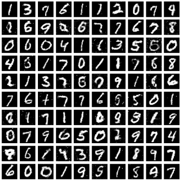
After 10 epochs of training with a batch size of 16 and a steps per epoch size of 3750, above are the results I got.
Not horrible, but there’s room to improve. Furthermore, if you try to run this on CIFAR-10, you will most likely get unusable results. An FCGAN won’t cut it. To fix that, we can use a DCGAN.

沒有留言:
張貼留言