Source From Here
Question
When you have just found out that you or a fellow team mate has committed sensitive data into your Github repo. What do you do? If you do not have hundreds of commits already. You can follow the steps mentioned below. Source: StackOverflow
WARNING: This should be used with care! It also removes the configuration of the repo.
How-To
Step 1
Remove all history
Step 2
Init a new repo
Step 3
Push to remote
Supplement
* 2.5 Git Basics - Working with Remotes
This is a blog to track what I had learned and share knowledge with all who can take advantage of them
標籤
- [ 英文學習 ]
- [ 計算機概論 ]
- [ 深入雲計算 ]
- [ 雜七雜八 ]
- [ Algorithm in Java ]
- [ Data Structures with Java ]
- [ IR Class ]
- [ Java 文章收集 ]
- [ Java 代碼範本 ]
- [ Java 套件 ]
- [ JVM 應用 ]
- [ LFD Note ]
- [ MangoDB ]
- [ Math CC ]
- [ MongoDB ]
- [ MySQL 小學堂 ]
- [ Python 考題 ]
- [ Python 常見問題 ]
- [ Python 範例代碼 ]
- [心得扎記]
- [網路教學]
- [C 常見考題]
- [C 範例代碼]
- [C/C++ 範例代碼]
- [Intro Alg]
- [Java 代碼範本]
- [Java 套件]
- [Linux 小技巧]
- [Linux 小學堂]
- [Linux 命令]
- [ML In Action]
- [ML]
- [MLP]
- [Postgres]
- [Python 學習筆記]
- [Quick Python]
- [Software Engineering]
- [The python tutorial]
- 工具收集
- 設計模式
- 資料結構
- ActiveMQ In Action
- AI
- Algorithm
- Android
- Ansible
- AWS
- Big Data 研究
- C/C++
- C++
- CCDH
- CI/CD
- Coursera
- Database
- DB
- Design Pattern
- Device Driver Programming
- Docker
- Docker 工具
- Docker Practice
- Eclipse
- English Writing
- ExtJS 3.x
- FP
- Fraud Prevention
- FreeBSD
- GCC
- Git
- Git Pro
- GNU
- Golang
- Gradle
- Groovy
- Hadoop
- Hadoop. Hadoop Ecosystem
- Java
- Java Framework
- Java UI
- JavaIDE
- JavaScript
- Jenkins
- JFreeChart
- Kaggle
- Kali/Metasploit
- Keras
- KVM
- Learn Spark
- LeetCode
- Linux
- Lucene
- Math
- ML
- ML Udemy
- Mockito
- MPI
- Nachos
- Network
- NLP
- node js
- OO
- OpenCL
- OpenMP
- OSC
- OSGi
- Pandas
- Perl
- PostgreSQL
- Py DS
- Python
- Python 自製工具
- Python Std Library
- Python tools
- QEMU
- R
- Real Python
- RIA
- RTC
- Ruby
- Ruby Packages
- Scala
- ScalaIA
- SQLAlchemy
- TensorFlow
- Tools
- UML
- Unix
- Verilog
- Vmware
- Windows 技巧
- wxPython
2020年7月30日 星期四
[Linux 常見問題] Compressing folders with password via command line
Source From Here
Question
I would like to know whether it is possible to do the following via CLI.
I have a Folder F which contains several sub folders and some files. I want to compress folder F into .zip file with the "password-only-extract".
How-To
Go to the relevant folder using the cd command like this:
(If your folder )
Then, type in your terminal:
This will prompt you for a password. Give it, and that will create a password-protected zip file from that folder.
There is an option called -P that will allow you to pass the password in the command itself, but that is not good because there is always the threat of over-the-shoulder peeking. Also other users can see the password by using ps -ef command if you use -P switch. With that -P switch, the command will look like this:
Visit man zip for more information.
Question
I would like to know whether it is possible to do the following via CLI.
I have a Folder F which contains several sub folders and some files. I want to compress folder F into .zip file with the "password-only-extract".
How-To
Go to the relevant folder using the cd command like this:
# cd /path/to/folder/
(If your folder )
Then, type in your terminal:
# zip -er F.zip F
This will prompt you for a password. Give it, and that will create a password-protected zip file from that folder.
* -e enables encryption for your zip file. This is what makes it ask for the password.
* -r makes the command recursive, meaning that all the files inside the folder will be added to the zip file.
* F.zip is the name of the output file.
* F is the folder you want to zip.
There is an option called -P that will allow you to pass the password in the command itself, but that is not good because there is always the threat of over-the-shoulder peeking. Also other users can see the password by using ps -ef command if you use -P switch. With that -P switch, the command will look like this:
# zip -P password -r F.zip F
Visit man zip for more information.
[Git 常見問題] How to delete remote branches in Git
Source From Here
Preface
While working with Git, it is possible that you come across a situation where you want to delete a remote branch. But before jumping into the intricacies of deleting a remote branch, let’s revisit how you would go about deleting a branch in the local repository with Git.
Deleting local branches
1. First, we print out all the branches (local as well as remote), using the git branch command with -a (all) flag.
2. To delete the local branch, just run the git branch command again, this time with the -d (delete) flag, followed by the name of the branch you want to delete (test branch in this case).
Note: Comments are the output produced as a result of running these git commands
Note: You can also use the -D flag which is synonymous with --delete --force instead of -d. This will delete the branch regardless of its merge status.
Deleting remote branches
To delete a remote branch, you can’t use the git branch command. Instead, use the git push command with --delete flag, followed by the name of the branch you want to delete. You also need to specify the remote name (origin in this case) after git push.
Preface
While working with Git, it is possible that you come across a situation where you want to delete a remote branch. But before jumping into the intricacies of deleting a remote branch, let’s revisit how you would go about deleting a branch in the local repository with Git.
Deleting local branches
1. First, we print out all the branches (local as well as remote), using the git branch command with -a (all) flag.
2. To delete the local branch, just run the git branch command again, this time with the -d (delete) flag, followed by the name of the branch you want to delete (test branch in this case).
Note: Comments are the output produced as a result of running these git commands
# git branch -a
*master
# git branch -d test
Deleted branch test (was ########).
Note: You can also use the -D flag which is synonymous with --delete --force instead of -d. This will delete the branch regardless of its merge status.
Deleting remote branches
To delete a remote branch, you can’t use the git branch command. Instead, use the git push command with --delete flag, followed by the name of the branch you want to delete. You also need to specify the remote name (origin in this case) after git push.
# git branch -a
*master
# git push origin --delete test
To <URL of your repository>.git
2020年7月8日 星期三
[Py DS] Ch5 - Machine Learning (Part14)
Application: A Face Detection Pipeline
This chapter has explored a number of the central concepts and algorithms of machine learning. But moving from these concepts to real-world application can be a challenge. Real-world datasets are noisy and heterogeneous, may have missing features, and may include data in a form that is difficult to map to a clean [n_samples, n_features] matrix. Before applying any of the methods discussed here, you must first extract these features from your data; there is no formula for how to do this that applies across all domains, and thus this is where you as a data scientist must exercise your own intuition and expertise.
One interesting and compelling application of machine learning is to images, and we have already seen a few examples of this where pixel-level features are used for classification. In the real world, data is rarely so uniform and simple pixels will not be suitable, a fact that has led to a large literature on feature extraction methods for image data (see “Feature Engineering” on page 375).
In this section, we will take a look at one such feature extraction technique, the Histogram of Oriented Gradients (HOG), which transforms image pixels into a vector representation that is sensitive to broadly informative image features regardless of confounding factors like illumination. We will use these features to develop a simple face detection pipeline, using machine learning algorithms and concepts we’ve seen throughout this chapter. We begin with the standard imports:
HOG Features
The Histogram of Gradients is a straightforward feature extraction procedure that was developed in the context of identifying pedestrians within images. HOG involves the following steps:
A fast HOG extractor is built into the Scikit-Image project, and we can try it out relatively quickly and visualize the oriented gradients within each cell (Figure 5-149):
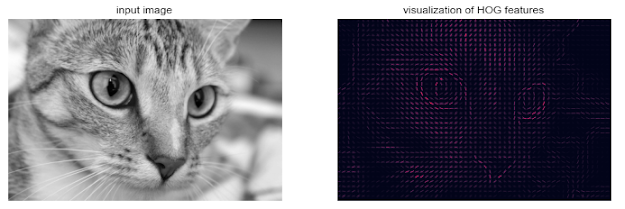
Figure 5-149. Visualization of HOG features computed from an image
HOG in Action: A Simple Face Detector
Using these HOG features, we can build up a simple facial detection algorithm with any Scikit-Learn estimator; here we will use a linear support vector machine (refer back to “In-Depth: Support Vector Machines” on page 405 if you need a refresher on this). The steps are as follows:
Let’s go through these steps and try it out:
1. Obtain a set of positive training samples.
Let’s start by finding some positive training samples that show a variety of faces. We have one easy set of data to work with—the Labeled Faces in the Wild dataset, which can be downloaded by Scikit-Learn:
Output:
This gives us a sample of 13,000 face images to use for training.
2. Obtain a set of negative training samples.
Next we need a set of similarly sized thumbnails that do not have a face in them. One way to do this is to take any corpus of input images, and extract thumbnails from them at a variety of scales. Here we can use some of the images shipped with Scikit-Image, along with Scikit-Learn’s PatchExtractor:
from skimage import data, transform
Output:
We now have 30,000 suitable image patches that do not contain faces. Let’s take a look at a few of them to get an idea of what they look like (Figure 5-150):
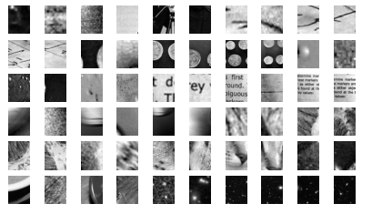
Figure 5-150. Negative image patches, which don’t include faces
Our hope is that these would sufficiently cover the space of “nonfaces” that our algorithm is likely to see.
3. Combine sets and extract HOG features.
Now that we have these positive samples and negative samples, we can combine them and compute HOG features. This step takes a little while, because the HOG features involve a nontrivial computation for each image:
Output:
We are left with 43,000 training samples in 1,215 dimensions, and we now have our data in a form that we can feed into Scikit-Learn!
4. Train a support vector machine
Next we use the tools we have been exploring in this chapter to create a classifier of thumbnail patches. For such a high-dimensional binary classification task, a linear support vector machine is a good choice. We will use Scikit-Learn’s LinearSVC, because in comparison to SVC it often has better scaling for large number of samples.
First, though, let’s use a simple Gaussian naive Bayes to get a quick baseline:
Output:
We see that on our training data, even a simple naive Bayes algorithm gets us upward of 90% accuracy. Let’s try the support vector machine, with a grid search over a few choices of the C parameter:
Output:
Output:
Let’s take the best estimator and retrain it on the full dataset:
5. Find faces in a new image.
Now that we have this model in place, let’s grab a new image and see how the model does. We will use one portion of the astronaut image for simplicity (see discussion of this in “Caveats and Improvements”), and run a sliding window over it and evaluate each patch (Figure 5-151):

Figure 5-151. An image in which we will attempt to locate a face
Next, let’s create a window that iterates over patches of this image, and compute HOG features for each patch:
Output:
Finally, we can take these HOG-featured patches and use our model to evaluate whether each patch contains a face:
Output:
We see that out of nearly 2,000 patches, we have found 51 detections. Let’s use the information we have about these patches to show where they lie on our test image, drawing them as rectangles (Figure 5-152):
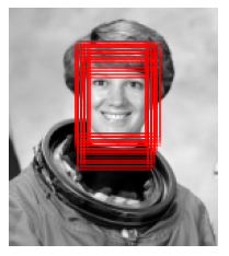
Figure 5-152. Windows that were determined to contain a face
All of the detected patches overlap and found the face in the image! Not bad for a few lines of Python.
Caveats and Improvements
If you dig a bit deeper into the preceding code and examples, you’ll see that we still have a bit of work before we can claim a production-ready face detector. There are several issues with what we’ve done, and several improvements that could be made. In particular:
Our training set, especially for negative features, is not very complete
Our current pipeline searches only at one scale
We should combine overlapped detection patches
The pipeline should be streamlined
More recent advances, such as deep learning, should be considered
Supplement
* Further Machine Learning Resources
This chapter has explored a number of the central concepts and algorithms of machine learning. But moving from these concepts to real-world application can be a challenge. Real-world datasets are noisy and heterogeneous, may have missing features, and may include data in a form that is difficult to map to a clean [n_samples, n_features] matrix. Before applying any of the methods discussed here, you must first extract these features from your data; there is no formula for how to do this that applies across all domains, and thus this is where you as a data scientist must exercise your own intuition and expertise.
One interesting and compelling application of machine learning is to images, and we have already seen a few examples of this where pixel-level features are used for classification. In the real world, data is rarely so uniform and simple pixels will not be suitable, a fact that has led to a large literature on feature extraction methods for image data (see “Feature Engineering” on page 375).
In this section, we will take a look at one such feature extraction technique, the Histogram of Oriented Gradients (HOG), which transforms image pixels into a vector representation that is sensitive to broadly informative image features regardless of confounding factors like illumination. We will use these features to develop a simple face detection pipeline, using machine learning algorithms and concepts we’ve seen throughout this chapter. We begin with the standard imports:
- %matplotlib inline
- import matplotlib.pyplot as plt
- import seaborn as sns; sns.set()
- import numpy as np
The Histogram of Gradients is a straightforward feature extraction procedure that was developed in the context of identifying pedestrians within images. HOG involves the following steps:
1. Optionally prenormalize images. This leads to features that resist dependence on variations in illumination.
2. Convolve the image with two filters that are sensitive to horizontal and vertical brightness gradients. These capture edge, contour, and texture information.
3. Subdivide the image into cells of a predetermined size, and compute a histogram of the gradient orientations within each cell.
4. Normalize the histograms in each cell by comparing to the block of neighboring cells. This further suppresses the effect of illumination across the image.
5. Construct a one-dimensional feature vector from the information in each cell.
A fast HOG extractor is built into the Scikit-Image project, and we can try it out relatively quickly and visualize the oriented gradients within each cell (Figure 5-149):
- from skimage import data, color, feature
- import skimage.data
- image = color.rgb2gray(data.chelsea())
- hog_vec, hog_vis = feature.hog(image, visualize=True)
- fig, ax = plt.subplots(1, 2, figsize=(12, 6),
- subplot_kw=dict(xticks=[], yticks=[]))
- ax[0].imshow(image, cmap='gray')
- ax[0].set_title('input image')
- ax[1].imshow(hog_vis)
- ax[1].set_title('visualization of HOG features');

Figure 5-149. Visualization of HOG features computed from an image
HOG in Action: A Simple Face Detector
Using these HOG features, we can build up a simple facial detection algorithm with any Scikit-Learn estimator; here we will use a linear support vector machine (refer back to “In-Depth: Support Vector Machines” on page 405 if you need a refresher on this). The steps are as follows:
1. Obtain a set of image thumbnails of faces to constitute “positive” training samples.
2. Obtain a set of image thumbnails of nonfaces to constitute “negative” training samples.
3. Extract HOG features from these training samples.
4. Train a linear SVM classifier on these samples.
5. For an “unknown” image, pass a sliding window across the image, using the model to evaluate whether that window contains a face or not.
6. If detections overlap, combine them into a single window.
Let’s go through these steps and try it out:
1. Obtain a set of positive training samples.
Let’s start by finding some positive training samples that show a variety of faces. We have one easy set of data to work with—the Labeled Faces in the Wild dataset, which can be downloaded by Scikit-Learn:
- from sklearn.datasets import fetch_lfw_people
- faces = fetch_lfw_people()
- positive_patches = faces.images
- positive_patches.shape
(13233, 62, 47)
This gives us a sample of 13,000 face images to use for training.
2. Obtain a set of negative training samples.
Next we need a set of similarly sized thumbnails that do not have a face in them. One way to do this is to take any corpus of input images, and extract thumbnails from them at a variety of scales. Here we can use some of the images shipped with Scikit-Image, along with Scikit-Learn’s PatchExtractor:
from skimage import data, transform
- imgs_to_use = ['camera', 'text', 'coins', 'moon', 'page', 'clock', 'immunohistochemistry',
- 'chelsea', 'coffee', 'hubble_deep_field']
- images = [color.rgb2gray(getattr(data, name)()) for name in imgs_to_use]
- from sklearn.feature_extraction.image import PatchExtractor
- def extract_patches(img, N, scale=1.0, patch_size=positive_patches[0].shape):
- extracted_patch_size = tuple((scale * np.array(patch_size)).astype(int))
- extractor = PatchExtractor(patch_size=extracted_patch_size, max_patches=N, random_state=0)
- patches = extractor.transform(img[np.newaxis])
- if scale != 1:
- patches = np.array([transform.resize(patch, patch_size) for patch in patches])
- return patches
- negative_patches = np.vstack([extract_patches(im, 1000, scale) for im in images for scale in [0.5, 1.0, 2.0]])
- negative_patches.shape
(30000, 62, 47)
We now have 30,000 suitable image patches that do not contain faces. Let’s take a look at a few of them to get an idea of what they look like (Figure 5-150):
- fig, ax = plt.subplots(6, 10)
- for i, axi in enumerate(ax.flat):
- axi.imshow(negative_patches[500 * i], cmap='gray')
- axi.axis('off')

Figure 5-150. Negative image patches, which don’t include faces
Our hope is that these would sufficiently cover the space of “nonfaces” that our algorithm is likely to see.
3. Combine sets and extract HOG features.
Now that we have these positive samples and negative samples, we can combine them and compute HOG features. This step takes a little while, because the HOG features involve a nontrivial computation for each image:
- from itertools import chain
- X_train = np.array([feature.hog(im) for im in chain(positive_patches, negative_patches)])
- y_train = np.zeros(X_train.shape[0])
- y_train[:positive_patches.shape[0]] = 1
- X_train.shape
(43233, 1215)
We are left with 43,000 training samples in 1,215 dimensions, and we now have our data in a form that we can feed into Scikit-Learn!
4. Train a support vector machine
Next we use the tools we have been exploring in this chapter to create a classifier of thumbnail patches. For such a high-dimensional binary classification task, a linear support vector machine is a good choice. We will use Scikit-Learn’s LinearSVC, because in comparison to SVC it often has better scaling for large number of samples.
First, though, let’s use a simple Gaussian naive Bayes to get a quick baseline:
- from sklearn.naive_bayes import GaussianNB
- from sklearn.model_selection import cross_val_score
- cross_val_score(GaussianNB(), X_train, y_train)
array([0.94726495, 0.97131953, 0.97189777, 0.97478603, 0.97455471])
We see that on our training data, even a simple naive Bayes algorithm gets us upward of 90% accuracy. Let’s try the support vector machine, with a grid search over a few choices of the C parameter:
- from sklearn.svm import LinearSVC
- from sklearn.model_selection import GridSearchCV
- grid = GridSearchCV(LinearSVC(), {'C': [1.0, 2.0, 4.0, 8.0]})
- grid.fit(X_train, y_train)
- grid.best_score_
0.9887354267133868
- grid.best_params_
{'C': 1.0}
Let’s take the best estimator and retrain it on the full dataset:
- model = grid.best_estimator_
- model.fit(X_train, y_train)
Now that we have this model in place, let’s grab a new image and see how the model does. We will use one portion of the astronaut image for simplicity (see discussion of this in “Caveats and Improvements”), and run a sliding window over it and evaluate each patch (Figure 5-151):
- test_image = skimage.data.astronaut()
- test_image = skimage.color.rgb2gray(test_image)
- test_image = skimage.transform.rescale(test_image, 0.5)
- test_image = test_image[:160, 40:180]
- plt.imshow(test_image, cmap='gray')
- plt.axis('off');

Figure 5-151. An image in which we will attempt to locate a face
Next, let’s create a window that iterates over patches of this image, and compute HOG features for each patch:
- def sliding_window(img, patch_size=positive_patches[0].shape, istep=2, jstep=2, scale=1.0):
- Ni, Nj = (int(scale * s) for s in patch_size)
- for i in range(0, img.shape[0] - Ni, istep):
- for j in range(0, img.shape[1] - Ni, jstep):
- patch = img[i:i + Ni, j:j + Nj]
- if scale != 1:
- patch = transform.resize(patch, patch_size)
- yield (i, j), patch
- indices, patches = zip(*sliding_window(test_image))
- patches_hog = np.array([feature.hog(patch) for patch in patches])
- patches_hog.shape
(1911, 1215)
Finally, we can take these HOG-featured patches and use our model to evaluate whether each patch contains a face:
- labels = model.predict(patches_hog)
- labels.sum()
51.0
We see that out of nearly 2,000 patches, we have found 51 detections. Let’s use the information we have about these patches to show where they lie on our test image, drawing them as rectangles (Figure 5-152):
- fig, ax = plt.subplots()
- ax.imshow(test_image, cmap='gray')
- ax.axis('off')
- Ni, Nj = positive_patches[0].shape
- indices = np.array(indices)
- for i, j in indices[labels == 1]:
- ax.add_patch(plt.Rectangle((j, i), Nj, Ni, edgecolor='red', alpha=0.3, lw=2, facecolor='none'))

Figure 5-152. Windows that were determined to contain a face
All of the detected patches overlap and found the face in the image! Not bad for a few lines of Python.
Caveats and Improvements
If you dig a bit deeper into the preceding code and examples, you’ll see that we still have a bit of work before we can claim a production-ready face detector. There are several issues with what we’ve done, and several improvements that could be made. In particular:
Our training set, especially for negative features, is not very complete
The central issue is that there are many face-like textures that are not in the training set, and so our current model is very prone to false positives. You can see this if you try out the preceding algorithm on the full astronaut image: the current model leads to many false detections in other regions of the image.
We might imagine addressing this by adding a wider variety of images to the negative training set, and this would probably yield some improvement. Another way to address this is to use a more directed approach, such as hard negative mining. In hard negative mining, we take a new set of images that our classifier has not seen, find all the patches representing false positives, and explicitly add them as negative instances in the training set before retraining the classifier.
Our current pipeline searches only at one scale
As currently written, our algorithm will miss faces that are not approximately 62×47 pixels. We can straightforwardly address this by using sliding windows of a variety of sizes, and resizing each patch using skimage.transform.resize before feeding it into the model. In fact, the sliding_window() utility used here is already built with this in mind.
We should combine overlapped detection patches
For a production-ready pipeline, we would prefer not to have 50 detections of the same face, but to somehow reduce overlapping groups of detections down to a single detection. This could be done via an unsupervised clustering approach (MeanShift Clustering is one good candidate for this), or via a procedural approach such as non maximum suppression, an algorithm common in machine vision.
The pipeline should be streamlined
Once we address these issues, it would also be nice to create a more streamlined pipeline for ingesting training images and predicting sliding-window outputs. This is where Python as a data science tool really shines: with a bit of work, we could take our prototype code and package it with a well-designed object oriented API that gives the user the ability to use this easily. I will leave this as a proverbial “exercise for the reader.”
More recent advances, such as deep learning, should be considered
Finally, I should add that HOG and other procedural feature extraction methods for images are no longer state-of-the-art techniques. Instead, many modern object detection pipelines use variants of deep neural networks. One way to think of neural networks is that they are an estimator that determines optimal feature extraction strategies from the data, rather than relying on the intuition of the user. An intro to these deep neural net methods is conceptually (and computationally!) beyond the scope of this section, although open tools like Google’s TensorFlow have recently made deep learning approaches much more accessible than they once were. As of the writing of this book, deep learning in Python is still relatively young, and so I can’t yet point to any definitive resource. That said, the list of references in the following section should provide a useful place to start.
Supplement
* Further Machine Learning Resources
訂閱:
意見 (Atom)
[Git 常見問題] error: The following untracked working tree files would be overwritten by merge
Source From Here 方案1: // x -----删除忽略文件已经对 git 来说不识别的文件 // d -----删除未被添加到 git 的路径中的文件 // f -----强制运行 # git clean -d -fx 方案2: 今天在服务器上 gi...
-
前言 : 為什麼程序管理這麼重要呢?這是因為: * 首先,本章一開始就談到的,我們在操作系統時的各項工作其實都是經過某個 PID 來達成的 (包括你的 bash 環境), 因此,能不能進行某項工作,就與該程序的權限有關了。 * 再來,如果您的 Linux 系統是個...
-
CNN 卷積神經網路簡介 STEP1. 卷積神經網路介紹 CNN 卷積神經網路可以分成兩大部分: * 影像的特徵提取 : 透過 Convolution 與 Max Pooling 提取影像特徵. * Fully connected Feedforward n...
-
來源自 這裡 說明 : split 是 Perl 中非常有用的函式之一,它可以將一個字串分割並將之置於陣列中。若無特別的指定,該函式亦使用 RE 與 $_ 變數 語法 : * split /PATTERN/,EXPR,LIMIT * split /...
