Source From Here
Preface
Collaborative Filtering is the most common technique used when it comes to building intelligent recommender systems that can learn to give better recommendations as more information about users is collected. Most websites like Amazon, YouTube, and Netflix use collaborative filtering as a part of their sophisticated recommendation systems. You can use this technique to build recommenders that give suggestions to a user on the basis of the likes and dislikes of similar users.
In this article, you’ll learn about:
What Is Collaborative Filtering?
Collaborative Filtering is a technique that can filter out items that a user might like on the basis of reactions by similar users.
It works by searching a large group of people and finding a smaller set of users with tastes similar to a particular user. It looks at the items they like and combines them to create a ranked list of suggestions. There are many ways to decide which users are similar and combine their choices to create a list of recommendations. This article will show you how to do that with Python.
The Dataset
To experiment with recommendation algorithms, you’ll need data that contains a set of items and a set of users who have reacted to some of the items. The reaction can be explicit (rating on a scale of 1 to 5, likes or dislikes) or implicit (viewing an item, adding it to a wish list, the time spent on an article).
While working with such data, you’ll mostly see it in the form of a matrix consisting of the reactions given by a set of users to some items from a set of items. Each row would contain the ratings given by a user, and each column would contain the ratings received by an item. A matrix with five users and five items could look like this:
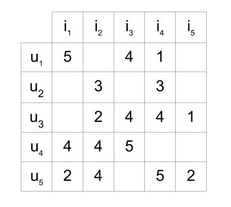
Rating Matrix
The matrix shows five users who have rated some of the items on a scale of 1 to 5. For example, the first user has given a rating 4 to the third item.
In most cases, the cells in the matrix are empty, as users only rate a few items. It’s highly unlikely for every user to rate or react to every item available. A matrix with mostly empty cells is called sparse, and the opposite to that (a mostly filled matrix) is called dense.
There are a lot of datasets that have been collected and made available to the public for research and benchmarking. Here’s a list of high-quality data sources that you can choose from.
The best one to get started would be the MovieLens dataset collected by GroupLens Research. In particular, the MovieLens 100k dataset is a stable benchmark dataset with 100,000 ratings given by 943 users for 1682 movies, with each user having rated at least 20 movies.
This dataset consists of many files that contain information about the movies, the users, and the ratings given by users to the movies they have watched. The ones that are of interest are the following:
The file u.data that contains the ratings is a tab separated list of user ID, item ID, rating, and timestamp. The first few lines of the file look like this:
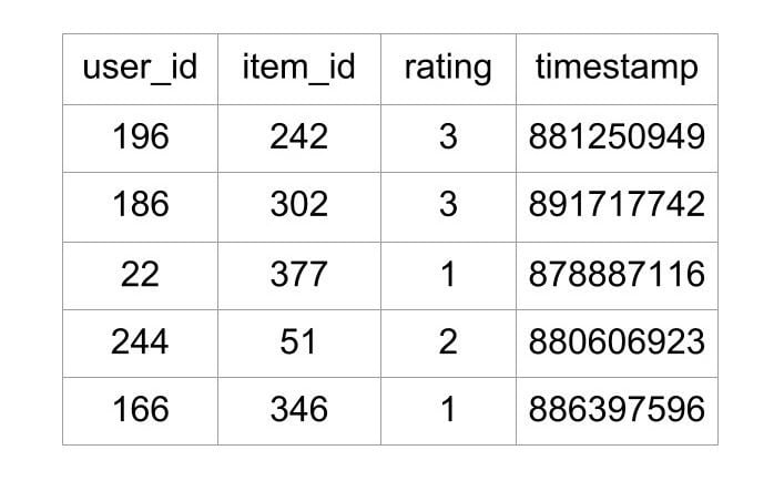
First 5 Rows of MovieLens 100k Data
As shown above, the file tells what rating a user gave to a particular movie. This file contains 100,000 such ratings, which will be used to predict the ratings of the movies not seen by the users.
Steps Involved in Collaborative Filtering
To build a system that can automatically recommend items to users based on the preferences of other users, the first step is to find similar users or items. The second step is to predict the ratings of the items that are not yet rated by a user. So, you will need the answers to these questions:
The first two questions don’t have single answers. Collaborative filtering is a family of algorithms where there are multiple ways to find similar users or items and multiple ways to calculate rating based on ratings of similar users. Depending on the choices you make, you end up with a type of collaborative filtering approach. You’ll get to see the various approaches to find similarity and predict ratings in this article.
One important thing to keep in mind is that in an approach based purely on collaborative filtering, the similarity is not calculated using factors like the age of users, genre of the movie, or any other data about users or items. It is calculated only on the basis of the rating (explicit or implicit) a user gives to an item. For example, two users can be considered similar if they give the same ratings to ten movies despite there being a big difference in their age.
The third question for how to measure the accuracy of your predictions also has multiple answers, which include error calculation techniques that can be used in many places and not just recommenders based on collaborative filtering.
One of the approaches to measure the accuracy of your result is the Root Mean Square Error (RMSE), in which you predict ratings for a test dataset of user-item pairs whose rating values are already known. The difference between the known value and the predicted value would be the error. Square all the error values for the test set, find the average (or mean), and then take the square root of that average to get the RMSE.
Another metric to measure the accuracy is Mean Absolute Error (MAE), in which you find the magnitude of error by finding its absolute value and then taking the average of all error values.
You don’t need to worry about the details of RMSE or MAE at this point as they are readily available as part of various packages in Python, and you will see them later in the article. Now let’s look at the different types of algorithms in the family of collaborative filtering.
Memory Based
The first category includes algorithms that are memory based, in which statistical techniques are applied to the entire dataset to calculate the predictions. To find the rating R that a user U would give to an item I, the approach includes:
How to Find Similar Users on the Basis of Ratings
To understand the concept of similarity, let’s create a simple dataset first. The data includes four users A, B, C, and D, who have rated two movies. The ratings are stored in lists, and each list contains two numbers indicating the rating of each movie:

Looking at the distance between the points seems to be a good way to estimate similarity, right? You can find the distance using the formula for Euclidean distance between two points. You can use the function available in scipy as shown in the following program:

As shown above, you can use scipy.spatial.distance.euclidean to calculate the distance between two points. So, what can you use to identify such patterns that Euclidean distance cannot? Can the angle between the lines joining the points to the origin be used to make a decision? You can take a look at the angle between the lines joining the origin of the graph to the respective points as shown:

The graph shows four lines joining each point to the origin. The lines for A and B are coincident, making the angle between them zero. You can consider that, if the angle between the lines is increased, then the similarity decreases, and if the angle is zero, then the users are very similar.
To calculate similarity using angle, you need a function that returns a higher similarity or smaller distance for a lower angle and a lower similarity or larger distance for a higher angle. The cosine of an angle is a function that decreases from 1 to -1 as the angle increases from 0 to 180.
You can use the cosine of the angle to find the similarity between two users. The higher the angle, the lower will be the cosine and thus, the lower will be the similarity of the users. You can also inverse the value of the cosine of the angle to get the cosine distance between the users by subtracting it from 1.
Scipy has a function spatial.distance.cosine that calculates the cosine distance of vectors. It returns a higher value for higher angle:

The lower angle between the vectors of C and A gives a lower cosine distance value. If you want to rank user similarities in this way, use cosine distance.
Notice that users A and B are considered absolutely similar in the cosine similarity metric despite having different ratings. This is actually a common occurrence in the real world, and the users like the user A are what you can call tough raters. An example would be a movie critic who always gives out ratings lower than the average, but the rankings of the items in their list would be similar to the Average raters like B.
To factor in such individual user preferences, you will need to bring all users to the same level by removing their biases. You can do this by subtracting the average rating given by that user to all items from each item rated by that user. Here’s what it would look like:
By doing this, you have changed the value of the average rating given by every user to 0. Try doing the same for users C and D, and you’ll see that the ratings are now adjusted to give an average of 0 for all users, which brings them all to the same level and removes their biases.
The cosine of the angle between the adjusted vectors is called centered cosine. This approach is normally used when there are a lot of missing values in the vectors, and you need to place a common value to fill up the missing values. Filling up the missing values in the ratings matrix with a random value could result in inaccuracies. A good choice to fill the missing values could be the average rating of each user, but the original averages of user A and B are 1.5 and 3 respectively, and filling up all the empty values of A with 1.5 and those of B with 3 would make them dissimilar users.
But after adjusting the values, the centered average of both users is 0, which allows you to capture the idea of the item being above or below average more accurately for both users with all missing values in both user’s vectors having the same value 0.
Euclidean distance and cosine similarity are some of the approaches that you can use to find users similar to one another and even items similar to one another. (The function used above calculates cosine distance. To calculate cosine similarity, subtract the distance from 1.)
How to Calculate the Ratings
After you have determined a list of users similar to a user U, you need to calculate the rating R that U would give to a certain item I. Again, just like similarity, you can do this in multiple ways. You can predict that a user’s rating R for an item I will be close to the average of the ratings given to I by the top 5 or top 10 users most similar to U. The mathematical formula for the average rating given by n users would look like this:

This formula shows that the average rating given by the n similar users is equal to the sum of the ratings given by them divided by the number of similar users, which is n.
There will be situations where the n similar users that you found are not equally similar to the target user U. The top 3 of them might be very similar, and the rest might not be as similar to U as the top 3. In that case, you could consider an approach where the rating of the most similar user matters more than the second most similar user and so on. The weighted average can help us achieve that.
In the weighted average approach, you multiply each rating by a similarity factor(which tells how similar the users are). By multiplying with the similarity factor, you add weights to the ratings. The heavier the weight, the more the rating would matter.
The similarity factor, which would act as weights, should be the inverse of the distance discussed above because less distance implies higher similarity. For example, you can subtract the cosine distance from 1 to get cosine similarity. With the similarity factor S for each user similar to the target user U, you can calculate the weighted average using this formula:

In the above formula, every rating is multiplied by the similarity factor of the user who gave the rating. The final predicted rating by user U will be equal to the sum of the weighted ratings divided by the sum of the weights. With a weighted average, you give more consideration to the ratings of similar users in order of their similarity.
Now, you know how to find similar users and how to calculate ratings based on their ratings. There’s also a variation of collaborative filtering where you predict ratings by finding items similar to each other instead of users and calculating the ratings. You’ll read about this variation in the next section.
User-Based vs Item-Based Collaborative Filtering
The technique in the examples explained above, where the rating matrix is used to find similar users based on the ratings they give, is called user-based or user-user collaborative filtering. If you use the rating matrix to find similar items based on the ratings given to them by users, then the approach is called item-based or item-item collaborative filtering.
The two approaches are mathematically quite similar, but there is a conceptual difference between the two. Here’s how the two compare:
- User-based
- Item-based
Item-based collaborative filtering was developed by Amazon. In a system where there are more users than items, item-based filtering is faster and more stable than user-based. It is effective because usually, the average rating received by an item doesn’t change as quickly as the average rating given by a user to different items. It’s also known to perform better than the user-based approach when the ratings matrix is sparse.
Although, the item-based approach performs poorly for datasets with browsing or entertainment related items such as MovieLens, where the recommendations it gives out seem very obvious to the target users. Such datasets see better results with matrix factorization techniques, which you’ll see in the next section, or with hybrid recommenders that also take into account the content of the data like the genre by using content-based filtering.
You can use the library Surprise to experiment with different recommender algorithms quickly. (You will see more about this later in the article.)
Model Based
The second category covers the Model based approaches, which involve a step to reduce or compress the large but sparse user-item matrix. For understanding this step, a basic understanding of dimensionality reduction can be very helpful.
Dimensionality Reduction
In the user-item matrix, there are two dimensions:
If the matrix is mostly empty, reducing dimensions can improve the performance of the algorithm in terms of both space and time. You can use various methods like matrix factorization or autoencoders to do this. Matrix factorization can be seen as breaking down a large matrix into a product of smaller ones. This is similar to the factorization of integers, where 12 can be written as 6 x 2 or 4 x 3. In the case of matrices, a matrix A with dimensions m x n can be reduced to a product of two matrices X and Y with dimensions m x p and p x n respectively.
The reduced matrices actually represent the users and items individually. The m rows in the first matrix represent the m users, and the p columns tell you about the features or characteristics of the users. The same goes for the item matrix with n items and p characteristics. Here’s an example of how matrix factorization looks:
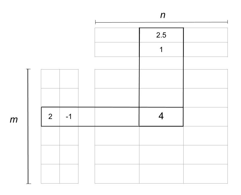
Matrix Factorization
In the image above, the matrix is reduced into two matrices. The one on the left is the user matrix with m users, and the one on top is the item matrix with n items. The rating 4 is reduced or factorized into:
The two columns in the user matrix and the two rows in the item matrix are called latent factors and are an indication of hidden characteristics about the users or the items. A possible interpretation of the factorization could look like this:
The factor matrices can provide such insights about users and items, but in reality they are usually much more complex than the explanation given above. The number of such factors can be anything from one to hundreds or even thousands. This number is one of the things that need to be optimized during the training of the model.
In the example, you had two latent factors for movie genres, but in real scenarios, these latent factors need not be analyzed too much. These are patterns in the data that will play their part automatically whether you decipher their underlying meaning or not. The number of latent factors affects the recommendations in a manner where the greater the number of factors, the more personalized the recommendations become. But too many factors can lead to overfitting in the model.
Algorithms for Matrix Factorization
One of the popular algorithms to factorize a matrix is the singular value decomposition (SVD) algorithm. SVD came into the limelight when matrix factorization was seen performing well in the Netflix prize competition. Other algorithms include PCA and its variations, NMF, and so on. Autoencoders can also be used for dimensionality reduction in case you want to use Neural Networks.
You can find the implementations of these algorithms in various libraries for Python so you don’t need to worry about the details at this point. But in case you want to read more, the chapter on dimensionality reduction in the book Mining of Massive Datasets is worth a read.
Using Python to Build Recommenders
There are quite a few libraries and toolkits in Python that provide implementations of various algorithms that you can use to build a recommender. But the one that you should try out while understanding recommendation systems is Surprise. Surprise is a Python SciKit that comes with various recommender algorithms and similarity metrics to make it easy to build and analyze recommenders.
Here’s how to install it using pip:
To use Surprise, you should first know some of the basic modules and classes available in it:
*The Dataset module is used to load data from files, Pandas dataframes, or even built-in datasets available for experimentation[/b] . (MovieLens 100k is one of the built-in datasets in Surprise.) To load a dataset, some of the available methods are:

* The Reader class is used to parse a file containing ratings. The default format in which it accepts data is that each rating is stored in a separate line in the order user item rating. This order and the separator can be configured using parameters:

Here’s a program that you can use to load data from a Pandas dataframe or the from builtin MovieLens 100k dataset:
- load_data.py
In the above program, the data is stored in a dictionary that is loaded into a Pandas dataframe and then into a Dataset object from Surprise.
Algorithms Based on K-Nearest Neighbours (k-NN)
The choice of algorithm for the recommender function depends on the technique you want to use. For the memory-based approaches discussed above, the algorithm that would fit the bill is Centered k-NN because the algorithm is very close to the centered cosine similarity formula explained above. It is available in Surprise as KNNWithMeans.
To find the similarity, you simply have to configure the function by passing a dictionary as an argument to the recommender function. The dictionary should have the required keys, such as the following:
The following program configures the KNNWithMeans function:
- recommender.py
The recommender function in the above program is configured to use the cosine similarity and to find similar items using the item-based approach.
To try out this recommender, you need to create a Trainset from data. Trainset is built using the same data but contains more information about the data, such as the number of users and items (n_users, n_items) that are used by the algorithm. You can create it either by using the entire data or a part of the data. You can also divide the data into folds where some of the data will be used for training and some for testing.
Here’s an example to find out how the user E would rate the movie 2:
The algorithm predicted that the user E would rate the movie 4.15, which could be high enough to be shown as a recommendation.
You should try out the different k-NN based algorithms along with different similarity options and matrix factorization algorithms available in the Surprise library. Try them out on the MovieLens dataset to see if you can beat some benchmarks. The next section will cover how to use Surprise to check which parameters perform best for your data.
Tuning the Algorithm Parameters
Surprise provides a GridSearchCV class analogous to GridSearchCV from scikit-learn.
With a dict of all parameters, GridSearchCV tries all the combinations of parameters and reports the best parameters for any accuracy measure For example, you can check which similarity metric works best for your data in memory-based approaches:
The output of the above program is as follows:
So, for the MovieLens 100k dataset, Centered-KNN algorithm works best if you go with item-based approach and use msd as the similarity metric with minimum support 3. Similarly, for model-based approaches, we can use Surprise to check which values for the following factors work best:
The following program will check the best values for the SVD algorithm, which is a matrix factorization algorithm:
The output of the above program is as follows:
So, for the MovieLens 100k dataset, the SVD algorithm works best if you go with 10 epochs and use a learning rate of 0.005 and 0.4 regularization. Other Matrix Factorization based algorithms available in Surprise are SVD++and NMF.
Following these examples, you can dive deep into all the parameters that can be used in these algorithms. You should definitely check out the mathematics behind them. Since you won’t have to worry much about the implementation of algorithms initially, recommenders can be a great way to segue into the field of machine learning and build an application based on that.
When Can Collaborative Filtering Be Used?
Collaborative filtering works around the interactions that users have with items. These interactions can help find patterns that the data about the items or users itself can’t. Here are some points that can help you decide if collaborative filtering can be used:
Although collaborative Filtering is very commonly used in recommenders, some of the challenges that are faced while using it are the following:
With every type of recommender algorithm having its own list of pros and cons, it’s usually a hybrid recommender that comes to the rescue. The benefits of multiple algorithms working together or in a pipeline can help you set up more accurate recommenders. In fact, the solution of the winner of the Netflix prize was also a complex mix of multiple algorithms.
Conclusion
You now know what calculations go into a collaborative-filtering type recommender and how to try out the various types of algorithms quickly on your dataset to see if collaborative filtering is the way to go. Even if it does not seem to fit your data with high accuracy, some of the use cases discussed might help you plan things in a hybrid way for the long term.
Here are some resources for more implementations and further reading on collaborative filtering and other recommendation algorithms:
- Libraries:
- Research papers:
* Item Based Collaborative Filtering Recommendation Algorithms: the first paper published on item-based recommenders
* Using collaborative filtering to weave an information tapestry: the first use of the term collaborative filtering
- Books:
Preface
Collaborative Filtering is the most common technique used when it comes to building intelligent recommender systems that can learn to give better recommendations as more information about users is collected. Most websites like Amazon, YouTube, and Netflix use collaborative filtering as a part of their sophisticated recommendation systems. You can use this technique to build recommenders that give suggestions to a user on the basis of the likes and dislikes of similar users.
In this article, you’ll learn about:
What Is Collaborative Filtering?
Collaborative Filtering is a technique that can filter out items that a user might like on the basis of reactions by similar users.
It works by searching a large group of people and finding a smaller set of users with tastes similar to a particular user. It looks at the items they like and combines them to create a ranked list of suggestions. There are many ways to decide which users are similar and combine their choices to create a list of recommendations. This article will show you how to do that with Python.
The Dataset
To experiment with recommendation algorithms, you’ll need data that contains a set of items and a set of users who have reacted to some of the items. The reaction can be explicit (rating on a scale of 1 to 5, likes or dislikes) or implicit (viewing an item, adding it to a wish list, the time spent on an article).
While working with such data, you’ll mostly see it in the form of a matrix consisting of the reactions given by a set of users to some items from a set of items. Each row would contain the ratings given by a user, and each column would contain the ratings received by an item. A matrix with five users and five items could look like this:
Rating Matrix
The matrix shows five users who have rated some of the items on a scale of 1 to 5. For example, the first user has given a rating 4 to the third item.
In most cases, the cells in the matrix are empty, as users only rate a few items. It’s highly unlikely for every user to rate or react to every item available. A matrix with mostly empty cells is called sparse, and the opposite to that (a mostly filled matrix) is called dense.
There are a lot of datasets that have been collected and made available to the public for research and benchmarking. Here’s a list of high-quality data sources that you can choose from.
The best one to get started would be the MovieLens dataset collected by GroupLens Research. In particular, the MovieLens 100k dataset is a stable benchmark dataset with 100,000 ratings given by 943 users for 1682 movies, with each user having rated at least 20 movies.
This dataset consists of many files that contain information about the movies, the users, and the ratings given by users to the movies they have watched. The ones that are of interest are the following:
The file u.data that contains the ratings is a tab separated list of user ID, item ID, rating, and timestamp. The first few lines of the file look like this:
First 5 Rows of MovieLens 100k Data
As shown above, the file tells what rating a user gave to a particular movie. This file contains 100,000 such ratings, which will be used to predict the ratings of the movies not seen by the users.
Steps Involved in Collaborative Filtering
To build a system that can automatically recommend items to users based on the preferences of other users, the first step is to find similar users or items. The second step is to predict the ratings of the items that are not yet rated by a user. So, you will need the answers to these questions:
The first two questions don’t have single answers. Collaborative filtering is a family of algorithms where there are multiple ways to find similar users or items and multiple ways to calculate rating based on ratings of similar users. Depending on the choices you make, you end up with a type of collaborative filtering approach. You’ll get to see the various approaches to find similarity and predict ratings in this article.
One important thing to keep in mind is that in an approach based purely on collaborative filtering, the similarity is not calculated using factors like the age of users, genre of the movie, or any other data about users or items. It is calculated only on the basis of the rating (explicit or implicit) a user gives to an item. For example, two users can be considered similar if they give the same ratings to ten movies despite there being a big difference in their age.
The third question for how to measure the accuracy of your predictions also has multiple answers, which include error calculation techniques that can be used in many places and not just recommenders based on collaborative filtering.
One of the approaches to measure the accuracy of your result is the Root Mean Square Error (RMSE), in which you predict ratings for a test dataset of user-item pairs whose rating values are already known. The difference between the known value and the predicted value would be the error. Square all the error values for the test set, find the average (or mean), and then take the square root of that average to get the RMSE.
Another metric to measure the accuracy is Mean Absolute Error (MAE), in which you find the magnitude of error by finding its absolute value and then taking the average of all error values.
You don’t need to worry about the details of RMSE or MAE at this point as they are readily available as part of various packages in Python, and you will see them later in the article. Now let’s look at the different types of algorithms in the family of collaborative filtering.
Memory Based
The first category includes algorithms that are memory based, in which statistical techniques are applied to the entire dataset to calculate the predictions. To find the rating R that a user U would give to an item I, the approach includes:
How to Find Similar Users on the Basis of Ratings
To understand the concept of similarity, let’s create a simple dataset first. The data includes four users A, B, C, and D, who have rated two movies. The ratings are stored in lists, and each list contains two numbers indicating the rating of each movie:
- from scipy import spatial
- import numpy as np
- import pandas as pd
- import matplotlib.pyplot as plt
- a = [1, 2]
- b = [2, 4]
- c = [2.5, 4]
- d = [4.5, 5]
- dot_names = ['A', 'B', 'C', 'D']
- dots = [a, b, c, d]
- x = list(map(lambda e: e[0], dots))
- y = list(map(lambda e: e[1], dots))
- fig, ax = plt.subplots()
- ax.scatter(x, y, alpha=0.5)
- ax.set_xlabel("Movie2", fontsize=15)
- ax.set_ylabel("Movie1", fontsize=15)
- ax.set_title('Rating of Movies')
- ax.grid(True)
- fig.tight_layout()
- for i, txt in enumerate(dot_names):
- ax.annotate(txt, (x[i], y[i]), fontsize=13)
- plt.show()
Looking at the distance between the points seems to be a good way to estimate similarity, right? You can find the distance using the formula for Euclidean distance between two points. You can use the function available in scipy as shown in the following program:
- dist_mtx = {}
- for i in range(len(dots)):
- dists = []
- for j in range(len(dots)):
- dists.append(spatial.distance.euclidean(dots[i], dots[j]))
- dist_mtx[dot_names[i]] = dists
- dist_df = pd.DataFrame(dist_mtx, index=dot_names)
- dist_df
As shown above, you can use scipy.spatial.distance.euclidean to calculate the distance between two points. So, what can you use to identify such patterns that Euclidean distance cannot? Can the angle between the lines joining the points to the origin be used to make a decision? You can take a look at the angle between the lines joining the origin of the graph to the respective points as shown:
- fig, ax = plt.subplots()
- for dot in dots:
- ax.plot([0, dot[0]], [0, dot[1]], 'bo-')
- for i, txt in enumerate(dot_names):
- ax.annotate(txt, (x[i], y[i] + 0.3), fontsize=13)
- ax.set_xlabel("Movie2", fontsize=15)
- ax.set_ylabel("Movie1", fontsize=15)
- ax.grid(True)
- plt.ylim(0, 6)
- fig.tight_layout()
- plt.show()
The graph shows four lines joining each point to the origin. The lines for A and B are coincident, making the angle between them zero. You can consider that, if the angle between the lines is increased, then the similarity decreases, and if the angle is zero, then the users are very similar.
To calculate similarity using angle, you need a function that returns a higher similarity or smaller distance for a lower angle and a lower similarity or larger distance for a higher angle. The cosine of an angle is a function that decreases from 1 to -1 as the angle increases from 0 to 180.
You can use the cosine of the angle to find the similarity between two users. The higher the angle, the lower will be the cosine and thus, the lower will be the similarity of the users. You can also inverse the value of the cosine of the angle to get the cosine distance between the users by subtracting it from 1.
Scipy has a function spatial.distance.cosine that calculates the cosine distance of vectors. It returns a higher value for higher angle:
- cos_dist_mtx = {}
- for i in range(len(dots)):
- dists = []
- for j in range(len(dots)):
- dists.append(spatial.distance.cosine(dots[i], dots[j]))
- dist_mtx[dot_names[i]] = dists
- dist_df = pd.DataFrame(dist_mtx, index=dot_names)
- dist_df
The lower angle between the vectors of C and A gives a lower cosine distance value. If you want to rank user similarities in this way, use cosine distance.
Notice that users A and B are considered absolutely similar in the cosine similarity metric despite having different ratings. This is actually a common occurrence in the real world, and the users like the user A are what you can call tough raters. An example would be a movie critic who always gives out ratings lower than the average, but the rankings of the items in their list would be similar to the Average raters like B.
To factor in such individual user preferences, you will need to bring all users to the same level by removing their biases. You can do this by subtracting the average rating given by that user to all items from each item rated by that user. Here’s what it would look like:
By doing this, you have changed the value of the average rating given by every user to 0. Try doing the same for users C and D, and you’ll see that the ratings are now adjusted to give an average of 0 for all users, which brings them all to the same level and removes their biases.
The cosine of the angle between the adjusted vectors is called centered cosine. This approach is normally used when there are a lot of missing values in the vectors, and you need to place a common value to fill up the missing values. Filling up the missing values in the ratings matrix with a random value could result in inaccuracies. A good choice to fill the missing values could be the average rating of each user, but the original averages of user A and B are 1.5 and 3 respectively, and filling up all the empty values of A with 1.5 and those of B with 3 would make them dissimilar users.
But after adjusting the values, the centered average of both users is 0, which allows you to capture the idea of the item being above or below average more accurately for both users with all missing values in both user’s vectors having the same value 0.
Euclidean distance and cosine similarity are some of the approaches that you can use to find users similar to one another and even items similar to one another. (The function used above calculates cosine distance. To calculate cosine similarity, subtract the distance from 1.)
How to Calculate the Ratings
After you have determined a list of users similar to a user U, you need to calculate the rating R that U would give to a certain item I. Again, just like similarity, you can do this in multiple ways. You can predict that a user’s rating R for an item I will be close to the average of the ratings given to I by the top 5 or top 10 users most similar to U. The mathematical formula for the average rating given by n users would look like this:
This formula shows that the average rating given by the n similar users is equal to the sum of the ratings given by them divided by the number of similar users, which is n.
There will be situations where the n similar users that you found are not equally similar to the target user U. The top 3 of them might be very similar, and the rest might not be as similar to U as the top 3. In that case, you could consider an approach where the rating of the most similar user matters more than the second most similar user and so on. The weighted average can help us achieve that.
In the weighted average approach, you multiply each rating by a similarity factor(which tells how similar the users are). By multiplying with the similarity factor, you add weights to the ratings. The heavier the weight, the more the rating would matter.
The similarity factor, which would act as weights, should be the inverse of the distance discussed above because less distance implies higher similarity. For example, you can subtract the cosine distance from 1 to get cosine similarity. With the similarity factor S for each user similar to the target user U, you can calculate the weighted average using this formula:

In the above formula, every rating is multiplied by the similarity factor of the user who gave the rating. The final predicted rating by user U will be equal to the sum of the weighted ratings divided by the sum of the weights. With a weighted average, you give more consideration to the ratings of similar users in order of their similarity.
Now, you know how to find similar users and how to calculate ratings based on their ratings. There’s also a variation of collaborative filtering where you predict ratings by finding items similar to each other instead of users and calculating the ratings. You’ll read about this variation in the next section.
User-Based vs Item-Based Collaborative Filtering
The technique in the examples explained above, where the rating matrix is used to find similar users based on the ratings they give, is called user-based or user-user collaborative filtering. If you use the rating matrix to find similar items based on the ratings given to them by users, then the approach is called item-based or item-item collaborative filtering.
The two approaches are mathematically quite similar, but there is a conceptual difference between the two. Here’s how the two compare:
- User-based
- Item-based
Item-based collaborative filtering was developed by Amazon. In a system where there are more users than items, item-based filtering is faster and more stable than user-based. It is effective because usually, the average rating received by an item doesn’t change as quickly as the average rating given by a user to different items. It’s also known to perform better than the user-based approach when the ratings matrix is sparse.
Although, the item-based approach performs poorly for datasets with browsing or entertainment related items such as MovieLens, where the recommendations it gives out seem very obvious to the target users. Such datasets see better results with matrix factorization techniques, which you’ll see in the next section, or with hybrid recommenders that also take into account the content of the data like the genre by using content-based filtering.
You can use the library Surprise to experiment with different recommender algorithms quickly. (You will see more about this later in the article.)
Model Based
The second category covers the Model based approaches, which involve a step to reduce or compress the large but sparse user-item matrix. For understanding this step, a basic understanding of dimensionality reduction can be very helpful.
Dimensionality Reduction
In the user-item matrix, there are two dimensions:
If the matrix is mostly empty, reducing dimensions can improve the performance of the algorithm in terms of both space and time. You can use various methods like matrix factorization or autoencoders to do this. Matrix factorization can be seen as breaking down a large matrix into a product of smaller ones. This is similar to the factorization of integers, where 12 can be written as 6 x 2 or 4 x 3. In the case of matrices, a matrix A with dimensions m x n can be reduced to a product of two matrices X and Y with dimensions m x p and p x n respectively.
The reduced matrices actually represent the users and items individually. The m rows in the first matrix represent the m users, and the p columns tell you about the features or characteristics of the users. The same goes for the item matrix with n items and p characteristics. Here’s an example of how matrix factorization looks:
Matrix Factorization
In the image above, the matrix is reduced into two matrices. The one on the left is the user matrix with m users, and the one on top is the item matrix with n items. The rating 4 is reduced or factorized into:
The two columns in the user matrix and the two rows in the item matrix are called latent factors and are an indication of hidden characteristics about the users or the items. A possible interpretation of the factorization could look like this:
The factor matrices can provide such insights about users and items, but in reality they are usually much more complex than the explanation given above. The number of such factors can be anything from one to hundreds or even thousands. This number is one of the things that need to be optimized during the training of the model.
In the example, you had two latent factors for movie genres, but in real scenarios, these latent factors need not be analyzed too much. These are patterns in the data that will play their part automatically whether you decipher their underlying meaning or not. The number of latent factors affects the recommendations in a manner where the greater the number of factors, the more personalized the recommendations become. But too many factors can lead to overfitting in the model.
Algorithms for Matrix Factorization
One of the popular algorithms to factorize a matrix is the singular value decomposition (SVD) algorithm. SVD came into the limelight when matrix factorization was seen performing well in the Netflix prize competition. Other algorithms include PCA and its variations, NMF, and so on. Autoencoders can also be used for dimensionality reduction in case you want to use Neural Networks.
You can find the implementations of these algorithms in various libraries for Python so you don’t need to worry about the details at this point. But in case you want to read more, the chapter on dimensionality reduction in the book Mining of Massive Datasets is worth a read.
Using Python to Build Recommenders
There are quite a few libraries and toolkits in Python that provide implementations of various algorithms that you can use to build a recommender. But the one that you should try out while understanding recommendation systems is Surprise. Surprise is a Python SciKit that comes with various recommender algorithms and similarity metrics to make it easy to build and analyze recommenders.
Here’s how to install it using pip:
To use Surprise, you should first know some of the basic modules and classes available in it:
*The Dataset module is used to load data from files, Pandas dataframes, or even built-in datasets available for experimentation[/b] . (MovieLens 100k is one of the built-in datasets in Surprise.) To load a dataset, some of the available methods are:
* The Reader class is used to parse a file containing ratings. The default format in which it accepts data is that each rating is stored in a separate line in the order user item rating. This order and the separator can be configured using parameters:
Here’s a program that you can use to load data from a Pandas dataframe or the from builtin MovieLens 100k dataset:
- load_data.py
- import pandas as pd
- from surprise import Dataset
- from surprise import Reader
- # This is the same data that was plotted for similarity earlier
- # with one new user "E" who has rated only movie 1
- ratings_dict = {
- "item": [1, 2, 1, 2, 1, 2, 1, 2, 1],
- "user": ['A', 'A', 'B', 'B', 'C', 'C', 'D', 'D', 'E'],
- "rating": [1, 2, 2, 4, 2.5, 4, 4.5, 5, 3],
- }
- df = pd.DataFrame(ratings_dict)
- reader = Reader(rating_scale=(1, 5))
- # Loads Pandas dataframe
- data = Dataset.load_from_df(df[["user", "item", "rating"]], reader)
- # Loads the builtin Movielens-100k data
- movielens = Dataset.load_builtin('ml-100k')
Algorithms Based on K-Nearest Neighbours (k-NN)
The choice of algorithm for the recommender function depends on the technique you want to use. For the memory-based approaches discussed above, the algorithm that would fit the bill is Centered k-NN because the algorithm is very close to the centered cosine similarity formula explained above. It is available in Surprise as KNNWithMeans.
To find the similarity, you simply have to configure the function by passing a dictionary as an argument to the recommender function. The dictionary should have the required keys, such as the following:
The following program configures the KNNWithMeans function:
- recommender.py
- from surprise import KNNWithMeans
- # To use item-based cosine similarity
- sim_options = {
- "name": "cosine",
- "user_based": False, # Compute similarities between items
- }
- algo = KNNWithMeans(sim_options=sim_options)
To try out this recommender, you need to create a Trainset from data. Trainset is built using the same data but contains more information about the data, such as the number of users and items (n_users, n_items) that are used by the algorithm. You can create it either by using the entire data or a part of the data. You can also divide the data into folds where some of the data will be used for training and some for testing.
Here’s an example to find out how the user E would rate the movie 2:
The algorithm predicted that the user E would rate the movie 4.15, which could be high enough to be shown as a recommendation.
You should try out the different k-NN based algorithms along with different similarity options and matrix factorization algorithms available in the Surprise library. Try them out on the MovieLens dataset to see if you can beat some benchmarks. The next section will cover how to use Surprise to check which parameters perform best for your data.
Tuning the Algorithm Parameters
Surprise provides a GridSearchCV class analogous to GridSearchCV from scikit-learn.
With a dict of all parameters, GridSearchCV tries all the combinations of parameters and reports the best parameters for any accuracy measure For example, you can check which similarity metric works best for your data in memory-based approaches:
- from surprise import KNNWithMeans
- from surprise import Dataset
- from surprise.model_selection import GridSearchCV
- data = Dataset.load_builtin("ml-100k")
- sim_options = {
- "name": ["msd", "cosine"],
- "min_support": [3, 4, 5],
- "user_based": [False, True],
- }
- param_grid = {"sim_options": sim_options}
- gs = GridSearchCV(KNNWithMeans, param_grid, measures=["rmse", "mae"], cv=3)
- gs.fit(data)
- print(gs.best_score["rmse"])
- print(gs.best_params["rmse"])
So, for the MovieLens 100k dataset, Centered-KNN algorithm works best if you go with item-based approach and use msd as the similarity metric with minimum support 3. Similarly, for model-based approaches, we can use Surprise to check which values for the following factors work best:
The following program will check the best values for the SVD algorithm, which is a matrix factorization algorithm:
- from surprise import SVD
- from surprise import Dataset
- from surprise.model_selection import GridSearchCV
- data = Dataset.load_builtin("ml-100k")
- param_grid = {
- "n_epochs": [5, 10],
- "lr_all": [0.002, 0.005],
- "reg_all": [0.4, 0.6]
- }
- gs = GridSearchCV(SVD, param_grid, measures=["rmse", "mae"], cv=3)
- gs.fit(data)
- print(gs.best_score["rmse"])
- print(gs.best_params["rmse"])
So, for the MovieLens 100k dataset, the SVD algorithm works best if you go with 10 epochs and use a learning rate of 0.005 and 0.4 regularization. Other Matrix Factorization based algorithms available in Surprise are SVD++and NMF.
Following these examples, you can dive deep into all the parameters that can be used in these algorithms. You should definitely check out the mathematics behind them. Since you won’t have to worry much about the implementation of algorithms initially, recommenders can be a great way to segue into the field of machine learning and build an application based on that.
When Can Collaborative Filtering Be Used?
Collaborative filtering works around the interactions that users have with items. These interactions can help find patterns that the data about the items or users itself can’t. Here are some points that can help you decide if collaborative filtering can be used:
Although collaborative Filtering is very commonly used in recommenders, some of the challenges that are faced while using it are the following:
With every type of recommender algorithm having its own list of pros and cons, it’s usually a hybrid recommender that comes to the rescue. The benefits of multiple algorithms working together or in a pipeline can help you set up more accurate recommenders. In fact, the solution of the winner of the Netflix prize was also a complex mix of multiple algorithms.
Conclusion
You now know what calculations go into a collaborative-filtering type recommender and how to try out the various types of algorithms quickly on your dataset to see if collaborative filtering is the way to go. Even if it does not seem to fit your data with high accuracy, some of the use cases discussed might help you plan things in a hybrid way for the long term.
Here are some resources for more implementations and further reading on collaborative filtering and other recommendation algorithms:
- Libraries:
- Research papers:
* Item Based Collaborative Filtering Recommendation Algorithms: the first paper published on item-based recommenders
* Using collaborative filtering to weave an information tapestry: the first use of the term collaborative filtering
- Books:


沒有留言:
張貼留言