[ FP with Java ] Ch6 - Dealing with optional data - Part2

Miscellaneous utilities for Option 
In order to make Option as useful as possible, you need to add some utility methods. Some of these methods are a must, and others are questionable because their use is not in the spirit of functional programming. You nevertheless must consider adding them. You may need a method to test whether an Option is a None or a Some. You may also need an equals method for comparing options, in which case you mustn’t forget to define a compatible hashCode method. 

Testing for Some or None 
Until now, you haven’t needed to test an option to know whether it was a Some or a None. Ideally, you should never have to do this. In practice, though, there are times when it’s simpler to use this trick than to resort to real functional techniques. For example, you defined the map2 method as: 

view plaincopy to clipboardprint?

1. Option map2(Option a,  
2.                          Option b,  
3.                          Function> f) {  
4.   return a.flatMap(ax -> b.map(bx -> f.apply(ax).apply(bx)));  
5. }  

This is very smart, and because you want to look smart, you might prefer this solution. But some may find the following version simpler to understand: 

view plaincopy to clipboardprint?

1. Option map2(Option a,  
2.                          Option b,  
3.                          Function> f) {  
4.   return a.isSome() && b.isSome()  
5.       ? some(f.apply(a.get()).apply(b.getOrThrow()))  
6.       : none();  
7. }  

Testing the Code 
If you want to test this code, you’ll have to define the isSome method first, but this is not to encourage you to use this nonfunctional technique. You should always prefer the first form, but you should also understand fully the relation between the two forms. Besides, you’ll probably find yourself needing the isSome method someday. 

equals and hashcode 
Much more important are the definitions of the equals and hashcode methods. As you know, these methods are strongly related and must be consistently defined. If equals is true for two instances of Option, their hashcode methods should return the same value. (The inverse is not true. Objects having the same hashcode may not always be equal.) Here are the implementations of equals and hashcode for Some: 

view plaincopy to clipboardprint?

1. @Override  
2. public boolean equals(Object o) {  
3.   return (this == o || o instanceof Some)  
4.                              && this.value.equals(((Some) o).value);  
5. }  
6.   
7. @Override  
8. public int hashCode() {  
9.   return Objects.hashCode(value);  
10. }  

And here are the corresponding implementations for None: 

view plaincopy to clipboardprint?

1. @Override  
2. public boolean equals(Object o) {  
3.   return this == o || o instanceof None;  
4. }  
5.   
6. @Override  
7. public int hashCode() {  
8.   return 0;  
9. }  

How and when to use Option 
As you may know, Java 8 has introduced the Optional class that may be seen by some as identical to your Option, although it’s not implemented in the same way at all, and it lacks most of the functional methods you’ve put into Option. There’s much controversy about whether the new features of Java 8 are a move toward functional programming. They certainly are, although this is not official. The official position is that Optional is not a functional feature. 

Here’s how Brian Goetz, Java language architect at Oracle, answered a question about this subject on Stack Overflow. The question was “Should Java 8 getters return optional types?” Here is Brian Goetz’s answer: 
The full discussion may be read at http://mng.bz/Rkk1. 

Of course, people will do what they want. But we did have a clear intention when adding this feature, and it was not to be a general purpose Maybe or Some type, as much as many people would have liked us to do so. Our intention was to provide a limited mechanism for library method return types where there needed to be a clear way to represent “no result” and using null for such was overwhelmingly likely to cause errors.

For example, you probably should never use it for something that returns an array of results, or a list of results; instead return an empty array or list. You should almost never use it as a field of something or a method parameter. I think routinely using it as a return value for getters would definitely be over-use. There’s nothing wrong with Optional that it should be avoided, it’s just not what many people wish it were, and accordingly we were fairly concerned about the risk of zealous over-use.

(Public service announcement: NEVER call Optional.get unless you can prove it will never be null; instead use one of the safe methods like orElse or ifPresent. In retrospect, we should have called get something like getOrElse-ThrowNoSuch-Element-Exception or something that made it far clearer that this was a highly dangerous method that undermined the whole purpose of Optional in the first place. Lesson learned.)

This is a very important answer that deserves some reflection. First of all, and this might be the most important part, “people will do what they want.” Nothing to add here. Just do what you want. This doesn’t mean you should do whatever you want without thinking. But feel free to try every solution that comes to mind. You shouldn’t refrain from using Optional in a particular way just because it wasn’t intended to be used that way. Imagine the first man who ever thought about grabbing a stone to hit something with more strength. He had two options (pun intended!): refraining from doing it because stones had obviously not been intended to be used as hammers, or just trying it. 

Second, Goetz says that get shouldn’t be called unless you can prove it will never be null. Doing this would completely ruin any benefit of using Option. But you don’t need to give get a very long name. getOrThrow would do the job. Note that returning an empty list to indicate the absence of a result doesn’t by itself solve the problem. Forgetting to test whether the list is empty will produce an IndexOutOfBoundException instead of a NullPointerException. Not much better! 

When to use getOrThrow 
The correct advice is to avoid getOrThrow as much as possible. As a rule of thumb, each time you find yourself using this method outside of the Option class, you should consider whether there’s another way to go. Using getOrThrow is exiting the functional safety of the Option class. 

The same thing is true for the head and tail methods of the List class. If possible, these methods shouldn’t be used outside of the List class. Directly accessing the value(s) contained in classes like List or Option always brings the risk of a NullPointerException if this is done on the None or Nil subclasses. It may not be possible to avoid in library classes, but it should be avoided in business classes. That’s why the best solution is to make this method protected, so that it can only be called from inside the Option class. 

But the most important point is the original question: should getters return Option (or Optional)? Generally, they shouldn’t, because properties should be final and initialized at declaration or in constructors, so there’s absolutely no need for getters to return Option. (I must admit, however, that initializing fields in constructors doesn’t guarantee that access to properties is impossible before they’re initialized. This is a marginal problem that’s easily solved by making classes final, if possible.) 

But some properties might be optional. For example, a person will always have a first name and a last name, but they might have no email. How can you represent this? By storing the property as an Option. In such cases, the getter will have to return an Option. Saying that “routinely using it as a return value for getters would definitely be over-use” is like saying that a property without a value should be set to null, and the corresponding getter should return null. This completely destroys the benefit of having Option. 

What about methods that take Option as their argument? In general, this should not occur. To compose methods returning Option, you shouldn’t use methods that take Option as their argument. For example, to compose the three following methods, you don’t need to change the methods to make them accept Option as their argument: 

view plaincopy to clipboardprint?

1. Option getName () {  
2.   ...  
3. }  
4.   
5. Option validate(String name) {  
6.   ...  
7. }  
8.   
9. Option getToon(String name) {  
10.   ...  
11. }  

Given that the validate method is a static method of class Validate, and toonMap is an instance of Map with the get instance method, the functional way to compose these methods is as follows: 

view plaincopy to clipboardprint?

1. Option toon = getName()  
2.                       .flatMap(Validate::validate)  
3.                       .flatMap(toonMap::get)  

So there’s little use for methods taking Option as parameters in business code. 

There’s another reason why Option (or Optional) should probably be used rarely (if ever). Generally, the absence of data is the result of errors that you should often handle by throwing an exception in imperative Java. As I said previously, returning Option.None instead of throwing an exception is like catching an exception and swallowing it silently. Usually it’s not a billion-dollar mistake, but it’s still a big one. You’ll learn in the next chapter how to deal with this situation. After that, you’ll hardly ever need the Option data type again. But don’t worry. All you’ve learned in this chapter will still be extremely useful. 

The Option type is the simplest form of a kind of data type that you’ll use again and again. It’s a parameterized type, it has a method to make an Option from an A, and it has a flatMap method that can be used to compose Optioninstances. Although it’s not very useful by itself, it has acquainted you with very fundamental concepts of functional programming. 

Supplement 
* FP with Java - Ch6 - Dealing with optional data - Part1 
* FP with Java - Ch6 - Dealing with optional data - Part2

[ ML 文章收集 ] Applied Deep Learning - Part 3: Autoencoders

Source From Here 

Overview 
Welcome to Part 3 of Applied Deep Learning series. Part 1 was a hands-on introduction to Artificial Neural Networks, covering both the theory and application with a lot of code examples and visualization. In Part 2 we applied deep learning to real-world datasets, covering the 3 most commonly encountered problems as case studies: binary classification, multiclass classification and regression. 

Now we will start diving into specific deep learning architectures, starting with the simplest: Autoencoders. The code for this article is available here as a Jupyter notebook, feel free to download and try it out yourself. 

Introduction 
Autoencoders are a specific type of feedforward neural networks where the input is the same as the output. They compress the input into a lower-dimensional code and then reconstruct the output from this representation. The code is a compact “summary” or “compression” of the input, also called the latent-space representation. 

An autoencoder consists of 3 components: encoder, code and decoder. The encoder compresses the input and produces the code, the decoder then reconstructs the input only using this code: 


To build an autoencoder we need 3 things: an encoding method, decoding method, and a loss function to compare the output with the target. We will explore these in the next section. Autoencoders are mainly a dimensionality reduction (or compression) algorithm with a couple of important properties: 

* Data-specific: Autoencoders are only able to meaningfully compress data similar to what they have been trained on. Since they learn features specific for the given training data, they are different than a standard data compression algorithm like gzip. So we can’t expect an autoencoder trained on handwritten digits to compress landscape photos.
* Lossy: The output of the autoencoder will not be exactly the same as the input, it will be a close but degraded representation. If you want lossless compression they are not the way to go.
* Unsupervised: To train an autoencoder we don’t need to do anything fancy, just throw the raw input data at it. Autoencoders are considered an unsupervised learning technique since they don’t need explicit labels to train on. But to be more precise they are self-supervised because they generate their own labels from the training data.

Architecture 
Let’s explore the details of the encoder, code and decoder. Both the encoder and decoder are fully-connected feedforward neural networks, essentially the ANNs we covered in Part 1. Code is a single layer of an ANN with the dimensionality of our choice. The number of nodes in the code layer (code size) is a hyperparameter that we set before training the autoencoder. 


This is a more detailed visualization of an autoencoder. First the input passes through the encoder, which is a fully-connected ANN, to produce the code. The decoder, which has the similar ANN structure, then produces the output only using the code. The goal is to get an output identical with the input. Note that the decoder architecture is the mirror image of the encoder. This is not a requirement but it’s typically the case. The only requirement is the dimensionality of the input and output needs to be the same. Anything in the middle can be played with. 

There are 4 hyperparameters that we need to set before training an autoencoder: 

* Code size: number of nodes in the middle layer. Smaller size results in more compression.
* Number of layers: the autoencoder can be as deep as we like. In the figure above we have 2 layers in both the encoder and decoder, without considering the input and output.
* Number of nodes per layer: the autoencoder architecture we’re working on is called a stacked autoencoder since the layers are stacked one after another. Usually stacked autoencoders look like a “sandwitch”. The number of nodes per layer decreases with each subsequent layer of the encoder, and increases back in the decoder. Also the decoder is symmetric to the encoder in terms of layer structure. As noted above this is not necessary and we have total control over these parameters.
* Loss function: we either use mean squared error (mse) or binary cross entropy. If the input values are in the range [0, 1] then we typically use crossentropy, otherwise we use the mean squared error. For more details check out this video.

Autoencoders are trained the same way as ANNs via backpropagation. Check out the introduction of Part 1 for more details on how neural networks are trained, it directly applies to the autoencoders. 

Implementation 
Now let’s implement an autoencoder for the following architecture, 1 hidden layer in the encoder and decoder. 


We will use the extremely popular MNIST dataset as input. It contains black-and-white images of handwritten digits. 

They’re of size 28x28 and we use them as a vector of 784 numbers between [0, 1]. Check the jupyter notebook for the details. We will now implement the autoencoder with Keras. The hyperparameters are: 128 nodes in the hidden layer, code size is 32, and binary crossentropy is the loss function: 

view plaincopy to clipboardprint?

1. input_size = 784  
2. hidden_size = 128  
3. code_size = 32  
4.   
5. input_img = Input(shape=(input_size,))  
6. hidden_1 = Dense(hidden_size, activation='relu')(input_img)  
7. code = Dense(code_size, activation='relu')(hidden_1)  
8. hidden_2 = Dense(hidden_size, activation='relu')(code)  
9. output_img = Dense(input_size, activation='sigmoid')(hidden_2)  
10.   
11. autoencoder = Model(input_img, output_img)  
12. autoencoder.compile(optimizer='adam', loss='binary_crossentropy')  
13. autoencoder.fit(x_train, x_train, epochs=5)  

This is very similar to the ANNs we worked on, but now we’re using the Keras functional API. Refer to this guide for details, but here’s a quick comparison. Before we used to add layers using the sequential API as follows: 

view plaincopy to clipboardprint?

1. model.add(Dense(16, activation='relu'))  
2. model.add(Dense(8, activation='relu'))  

With the functional API we do this: 

view plaincopy to clipboardprint?

1. layer_1 = Dense(16, activation='relu')(input)  
2. layer_2 = Dense(8, activation='relu')(layer_1)  

It’s more verbose but a more flexible way to define complex models. We can easily grab parts of our model, for example only the decoder, and work with that. The output of Dense method is a callable layer, using the functional API we provide it with the input and store the output. The output of a layer becomes the input of the next layer. With the sequential API the add method implicitly handled this for us. 

Note that all the layers use the Relu activation function, as it’s the standard with deep neural networks. The last layer uses the sigmoid activation because we need the outputs to be between [0, 1]. The input is also in the same range. Also note the call to fit function, before with ANNs we used to do: 

view plaincopy to clipboardprint?

1. model.fit(x_train, y_train)  

But now we do: 

view plaincopy to clipboardprint?

1. model.fit(x_train, x_train)  

Remember that the targets of the autoencoder are the same as the input. That’s why we supply the training data as the target. 

Visualization 
Now let’s visualize how well our autoencoder reconstructs its input. 

view plaincopy to clipboardprint?

1. reconstructed = autoencoder.predict(x_test)  

We run the autoencoder on the test set simply by using the predict function of Keras. For every image in the test set, we get the output of the autoencoder. We expect the output to be very similar to the input. 

They are indeed pretty similar, but not exactly the same. We can notice it more clearly in the last digit “4”. Since this was a simple task our autoencoder performed pretty well. 

Advice 
We have total control over the architecture of the autoencoder. We can make it very powerful by increasing the number of layers, nodes per layer and most importantly the code size. Increasing these hyperparameters will let the autoencoder to learn more complex codings. But we should be careful to not make it too powerful. Otherwise the autoencoder will simply learn to copy its inputs to the output, without learning any meaningful representation. It will just mimic the identity function. The autoencoder will reconstruct the training data perfectly, but it will be overfitting without being able to generalize to new instances, which is not what we want. 

This is why we prefer a “sandwitch” architecture, and deliberately keep the code size small. Since the coding layer has a lower dimensionality than the input data, the autoencoder is said to be undercomplete. It won’t be able to directly copy its inputs to the output, and will be forced to learn intelligent features. If the input data has a pattern, for example the digit “1” usually contains a somewhat straight line and the digit “0” is circular, it will learn this fact and encode it in a more compact form. If the input data was completely random without any internal correlation or dependency, then an undercomplete autoencoder won’t be able to recover it perfectly. But luckily in the real-world there is a lot of dependency. 

Denoising Autoencoders 
Keeping the code layer small forced our autoencoder to learn an intelligent representation of the data. There is another way to force the autoencoder to learn useful features, which is adding random noise to its inputs and making it recover the original noise-free data. This way the autoencoder can’t simply copy the input to its output because the input also contains random noise. We are asking it to subtract the noise and produce the underlying meaningful data. This is called a denoising autoencoder. 


The top row contains the original images. We add random Gaussian noise to them and the noisy data becomes the input to the autoencoder. The autoencoder doesn’t see the original image at all. But then we expect the autoencoder to regenerate the noise-free original image. 


There is only one small difference between the implementation of denoising autoencoder and the regular one. The architecture doesn’t change at all, only the fit function. We trained the regular autoencoder as follows: 

view plaincopy to clipboardprint?

1. autoencoder.fit(x_train, x_train)  

Denoising autoencoder is trained as: 

view plaincopy to clipboardprint?

1. autoencoder.fit(x_train_noisy, x_train)  

Simple as that, everything else is exactly the same. The input to the autoencoder is the noisy image, and the expected target is the original noise-free one. 

Visualization 
Now let’s visualize whether we are able to recover the noise-free images. 


Looks pretty good. The bottom row is the autoencoder output. We can do better by using more complex autoencoder architecture, such as convolutional autoencoders. We will cover convolutions in the upcoming article. 

Sparse Autoencoders 
We introduced two ways to force the autoencoder to learn useful features: keeping the code size small and denoising autoencoders. The third method is using regularization. We can regularize the autoencoder by using a sparsity constraint such that only a fraction of the nodes would have nonzero values, called active nodes. 

In particular, we add a penalty term to the loss function such that only a fraction of the nodes become active. This forces the autoencoder to represent each input as a combination of small number of nodes, and demands it to discover interesting structure in the data. This method works even if the code size is large, since only a small subset of the nodes will be active at any time. 

It’s pretty easy to do this in Keras with just one parameter. As a reminder, previously we created the code layer as follows: 

view plaincopy to clipboardprint?

1. code = Dense(code_size, activation='relu')(input_img)  

We now add another parameter called activity_regularizer by specifying the regularization strength. This is typically a value in the range [0.001, 0.000001]. Here we chose 10e-6. 

view plaincopy to clipboardprint?

1. code = Dense(code_size, activation='relu', activity_regularizer=l1(10e-6))(input_img)  

The final loss of the sparse model is 0.01 higher than the standard one, due to the added regularization term. 

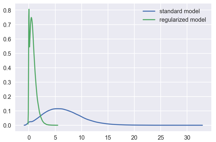
Let’s demonstrate the encodings generated by the regularized model are indeed sparse. If we look at the histogram of code values for the images in the test set, the distribution is as follows: 
 

The mean for the standard model is 6.6 but for the regularized model it’s 0.8, a pretty big reduction. We can see that a large chunk of code values in the regularized model are indeed 0, which is what we wanted. The variance of the regularized model is also fairly low. 

Use Cases 
Now we might ask the following questions. How good are autoencoders at compressing the input? And are they a commonly used deep learning technique? 

Unfortunately autoencoders are not widely used in real-world applications. As a compression method, they don’t perform better than its alternatives, for example jpeg does photo compression better than an autoencoder. And the fact that autoencoders are data-specific makes them impractical as a general technique. They have 3 common use cases though: 

* Data denoising: we have seen an example of this on images.
* Dimensionality reduction: visualizing high-dimensional data is challenging. t-SNE is the most commonly used method but struggles with large number of dimensions (typically above 32). So autoencoders are used as a preprocessing step to reduce the dimensionality, and this compressed representation is used by t-SNE to visualize the data in 2D space. For great articles on t-SNE refer here and here.
* Variational Autoencoders (VAE): this is a more modern and complex use-case of autoencoders and we will cover them in another article. But as a quick summary, VAE learns the parameters of the probability distribution modeling the input data, instead of learning an arbitrary function in the case of vanilla autoencoders. By sampling points from this distribution we can also use the VAE as a generative model. Here is a good reference.

Conclusion 
Autoencoders are a very useful dimensionality reduction technique. They are very popular as a teaching material in introductory deep learning courses, most likely due to their simplicity. In this article we covered them in detail and I hope you enjoyed it. The entire code for this article is available here if you want to hack on it yourself. If you have any feedback feel free to reach out to me on twitter. 

Supplement 
* ML Lecture 16: Unsupervised Learning - Auto-encoder 
* Applied Deep Learning - Part 1: Artificial Neural Networks 
* Applied Deep Learning - Part 2: Real World Case Studies