Source From Here
Overview Welcome to Part 3 of Applied Deep Learning series. Part 1 was a hands-on introduction to Artificial Neural Networks, covering both the theory and application with a lot of code examples and visualization. In Part 2 we applied deep learning to real-world datasets, covering the 3 most commonly encountered problems as case studies: binary classification, multiclass classification and regression.
Now we will start diving into specific deep learning architectures, starting with the simplest: Autoencoders. The code for this article is available here as a Jupyter notebook, feel free to download and try it out yourself.
Introduction
Autoencoders are a specific type of feedforward neural networks where the input is the same as the output. They compress the input into a lower-dimensional code and then reconstruct the output from this representation. The code is a compact “summary” or “compression” of the input, also called the latent-space representation.
An autoencoder consists of 3 components: encoder, code and decoder. The encoder compresses the input and produces the code, the decoder then reconstructs the input only using this code:

To build an autoencoder we need 3 things: an encoding method, decoding method, and a loss function to compare the output with the target. We will explore these in the next section. Autoencoders are mainly a dimensionality reduction (or compression) algorithm with a couple of important properties:
Architecture
Let’s explore the details of the encoder, code and decoder. Both the encoder and decoder are fully-connected feedforward neural networks, essentially the ANNs we covered in Part 1. Code is a single layer of an ANN with the dimensionality of our choice. The number of nodes in the code layer (code size) is a hyperparameter that we set before training the autoencoder.

This is a more detailed visualization of an autoencoder. First the input passes through the encoder, which is a fully-connected ANN, to produce the code. The decoder, which has the similar ANN structure, then produces the output only using the code. The goal is to get an output identical with the input. Note that the decoder architecture is the mirror image of the encoder. This is not a requirement but it’s typically the case. The only requirement is the dimensionality of the input and output needs to be the same. Anything in the middle can be played with.
There are 4 hyperparameters that we need to set before training an autoencoder:
Autoencoders are trained the same way as ANNs via backpropagation. Check out the introduction of Part 1 for more details on how neural networks are trained, it directly applies to the autoencoders.
Implementation
Now let’s implement an autoencoder for the following architecture, 1 hidden layer in the encoder and decoder.

We will use the extremely popular MNIST dataset as input. It contains black-and-white images of handwritten digits.

They’re of size 28x28 and we use them as a vector of 784 numbers between [0, 1]. Check the jupyter notebook for the details. We will now implement the autoencoder with Keras. The hyperparameters are: 128 nodes in the hidden layer, code size is 32, and binary crossentropy is the loss function:
- input_size = 784
- hidden_size = 128
- code_size = 32
- input_img = Input(shape=(input_size,))
- hidden_1 = Dense(hidden_size, activation='relu')(input_img)
- code = Dense(code_size, activation='relu')(hidden_1)
- hidden_2 = Dense(hidden_size, activation='relu')(code)
- output_img = Dense(input_size, activation='sigmoid')(hidden_2)
- autoencoder = Model(input_img, output_img)
- autoencoder.compile(optimizer='adam', loss='binary_crossentropy')
- autoencoder.fit(x_train, x_train, epochs=5)
- model.add(Dense(16, activation='relu'))
- model.add(Dense(8, activation='relu'))
- layer_1 = Dense(16, activation='relu')(input)
- layer_2 = Dense(8, activation='relu')(layer_1)
Note that all the layers use the Relu activation function, as it’s the standard with deep neural networks. The last layer uses the sigmoid activation because we need the outputs to be between [0, 1]. The input is also in the same range. Also note the call to fit function, before with ANNs we used to do:
- model.fit(x_train, y_train)
- model.fit(x_train, x_train)
Visualization
Now let’s visualize how well our autoencoder reconstructs its input.
- reconstructed = autoencoder.predict(x_test)
We run the autoencoder on the test set simply by using the predict function of Keras. For every image in the test set, we get the output of the autoencoder. We expect the output to be very similar to the input.

They are indeed pretty similar, but not exactly the same. We can notice it more clearly in the last digit “4”. Since this was a simple task our autoencoder performed pretty well.
Advice
We have total control over the architecture of the autoencoder. We can make it very powerful by increasing the number of layers, nodes per layer and most importantly the code size. Increasing these hyperparameters will let the autoencoder to learn more complex codings. But we should be careful to not make it too powerful. Otherwise the autoencoder will simply learn to copy its inputs to the output, without learning any meaningful representation. It will just mimic the identity function. The autoencoder will reconstruct the training data perfectly, but it will be overfitting without being able to generalize to new instances, which is not what we want.
This is why we prefer a “sandwitch” architecture, and deliberately keep the code size small. Since the coding layer has a lower dimensionality than the input data, the autoencoder is said to be undercomplete. It won’t be able to directly copy its inputs to the output, and will be forced to learn intelligent features. If the input data has a pattern, for example the digit “1” usually contains a somewhat straight line and the digit “0” is circular, it will learn this fact and encode it in a more compact form. If the input data was completely random without any internal correlation or dependency, then an undercomplete autoencoder won’t be able to recover it perfectly. But luckily in the real-world there is a lot of dependency.
Denoising Autoencoders
Keeping the code layer small forced our autoencoder to learn an intelligent representation of the data. There is another way to force the autoencoder to learn useful features, which is adding random noise to its inputs and making it recover the original noise-free data. This way the autoencoder can’t simply copy the input to its output because the input also contains random noise. We are asking it to subtract the noise and produce the underlying meaningful data. This is called a denoising autoencoder.

The top row contains the original images. We add random Gaussian noise to them and the noisy data becomes the input to the autoencoder. The autoencoder doesn’t see the original image at all. But then we expect the autoencoder to regenerate the noise-free original image.

There is only one small difference between the implementation of denoising autoencoder and the regular one. The architecture doesn’t change at all, only the fit function. We trained the regular autoencoder as follows:
- autoencoder.fit(x_train, x_train)
- autoencoder.fit(x_train_noisy, x_train)
Visualization
Now let’s visualize whether we are able to recover the noise-free images.

Looks pretty good. The bottom row is the autoencoder output. We can do better by using more complex autoencoder architecture, such as convolutional autoencoders. We will cover convolutions in the upcoming article.
Sparse Autoencoders
We introduced two ways to force the autoencoder to learn useful features: keeping the code size small and denoising autoencoders. The third method is using regularization. We can regularize the autoencoder by using a sparsity constraint such that only a fraction of the nodes would have nonzero values, called active nodes.
In particular, we add a penalty term to the loss function such that only a fraction of the nodes become active. This forces the autoencoder to represent each input as a combination of small number of nodes, and demands it to discover interesting structure in the data. This method works even if the code size is large, since only a small subset of the nodes will be active at any time.
It’s pretty easy to do this in Keras with just one parameter. As a reminder, previously we created the code layer as follows:
- code = Dense(code_size, activation='relu')(input_img)
- code = Dense(code_size, activation='relu', activity_regularizer=l1(10e-6))(input_img)
Let’s demonstrate the encodings generated by the regularized model are indeed sparse. If we look at the histogram of code values for the images in the test set, the distribution is as follows:
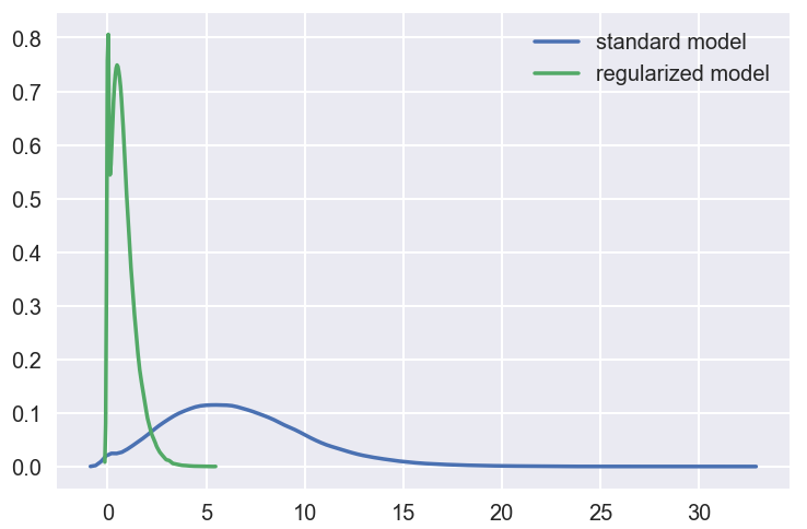
The mean for the standard model is 6.6 but for the regularized model it’s 0.8, a pretty big reduction. We can see that a large chunk of code values in the regularized model are indeed 0, which is what we wanted. The variance of the regularized model is also fairly low.
Use Cases
Now we might ask the following questions. How good are autoencoders at compressing the input? And are they a commonly used deep learning technique?
Unfortunately autoencoders are not widely used in real-world applications. As a compression method, they don’t perform better than its alternatives, for example jpeg does photo compression better than an autoencoder. And the fact that autoencoders are data-specific makes them impractical as a general technique. They have 3 common use cases though:
Conclusion
Autoencoders are a very useful dimensionality reduction technique. They are very popular as a teaching material in introductory deep learning courses, most likely due to their simplicity. In this article we covered them in detail and I hope you enjoyed it. The entire code for this article is available here if you want to hack on it yourself. If you have any feedback feel free to reach out to me on twitter.
Supplement
* ML Lecture 16: Unsupervised Learning - Auto-encoder
* Applied Deep Learning - Part 1: Artificial Neural Networks
* Applied Deep Learning - Part 2: Real World Case Studies

沒有留言:
張貼留言